Malcolm Low | Practical AI, Computing & Quantum Research

Singapore-based practical guides, tutorials and experiments in AI, computing, modelling, simulation, optimisation and quantum computing, with research notes and hands-on workflows.

Bloch Sphere Simulator: 3D Qubit State Visualizer Live

Interactive Quantum Tool • Module 2

Interactive 3D Bloch Sphere Simulator

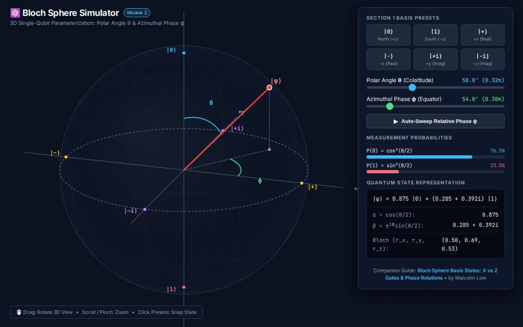
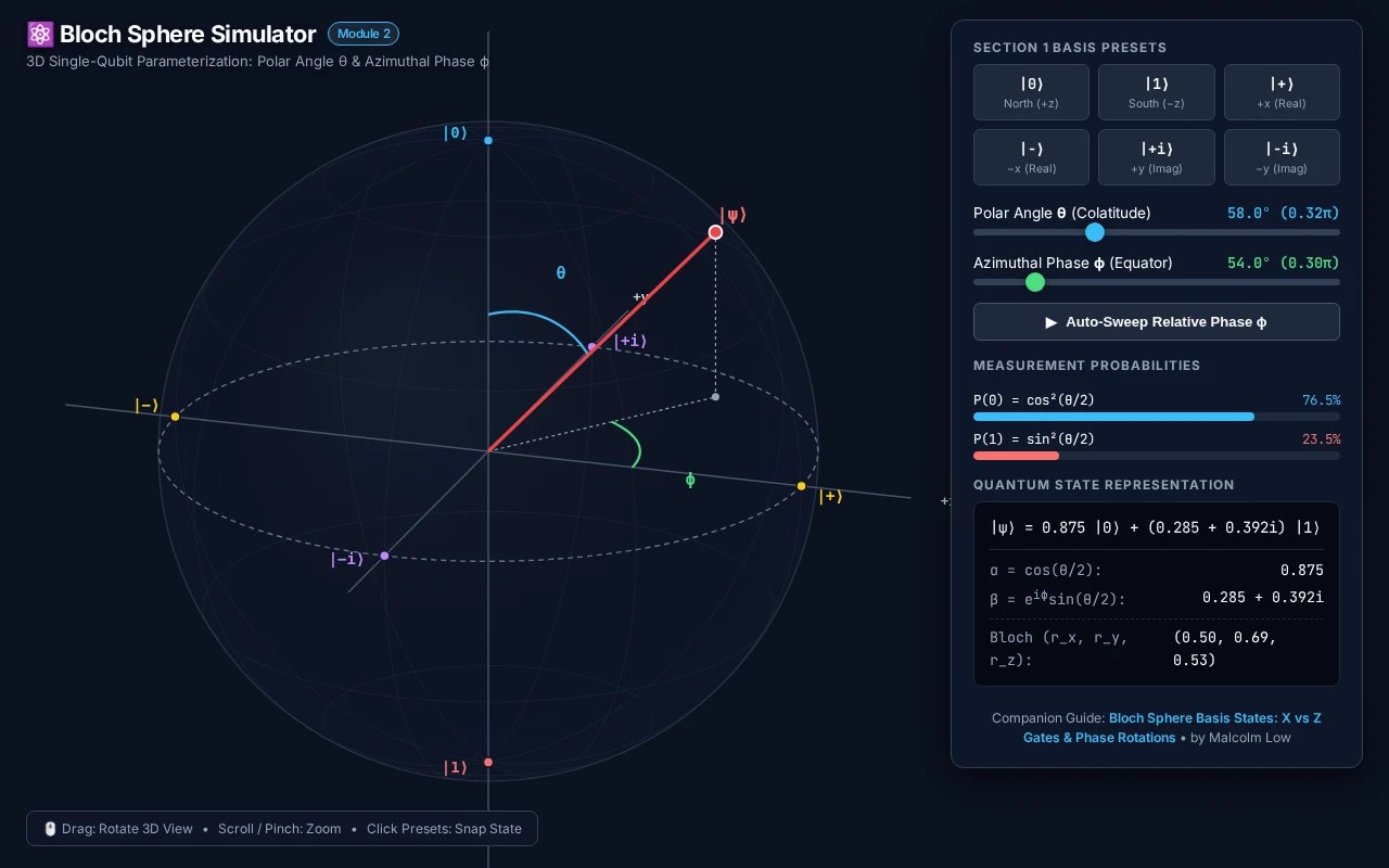
Explore single-qubit quantum states, polar angle θ, azimuthal relative phase ϕ, and basis state projections in real time with this interactive 3D WebGL/Canvas visualizer. Drag to orbit the sphere, adjust continuous angles, and instantly observe quantum measurement probabilities.

Interactive 3D Bloch Sphere Simulator Interface

Figure 1: The Interactive 3D Bloch Sphere Simulator interface showing state vector |ψ⟩, polar angle θ (blue arc), azimuthal phase ϕ (green arc), and real-time quantum measurement probabilities.

1. Spatial Anatomy & Controls Mapping

Based directly on Section 1 of our guide, Bloch Sphere Basis States: X vs Z Gates & Phase Rotations, the simulator maps the Hilbert space of a pure two-level quantum system to a 3D unit sphere surface:

  • The Computational Basis Poles: The North Pole (+z) marks ground state |0⟩ (θ = 0), while the South Pole (−z) marks excited state |1⟩ (θ = π).
  • The Hadamard Superposition Axis: Pierces the equator along the real axis (x). The positive +x direction represents the symmetric superposition |+⟩ = (|0⟩ + |1⟩)/√2 (θ = π/2, ϕ = 0), while −x represents |−⟩ = (|0⟩ − |1⟩)/√2 (θ = π/2, ϕ = π).
  • The Circular Phase Axis: Pierces the equator along the imaginary axis (y). The positive +y direction represents |+i⟩ = (|0⟩ + i|1⟩)/√2 (θ = π/2, ϕ = π/2), while −y represents |−i⟩ = (|0⟩ − i|1⟩)/√2 (θ = π/2, ϕ = 3π/2).

2. Hands-On Exploration Exercises

To build intuition for single-qubit quantum state parameterization, follow this recommended sequence inside the simulator:

  1. Verify Bit-Flip Inversion: Click the |0⟩ preset, then move the θ slider from 0° to 180°. Observe how P(0) smoothly decreases from 100% to 0% while P(1) increases from 0% to 100%, exactly tracking P(0) = cos²(θ/2).
  2. Equatorial 50/50 Invariance: Set θ = 90° (the equator). Notice that P(0) = 50.0% and P(1) = 50.0%. Now click Auto-Sweep Relative Phase ϕ. As the state vector completes a full 360° loop through |+⟩, |+i⟩, |−⟩, and |−i⟩, the computational measurement probabilities never change.
  3. Complex Phase Detection: Compare |+⟩ (ϕ = 0) and |−⟩ (ϕ = 180°). In the computational Z-basis, both yield identical measurement outcomes (50% 0, 50% 1). But in the 3D geometry, they sit antipodal across the sphere (r_x = +1 vs r_x = −1), requiring a basis rotation (Hadamard gate) to convert this relative phase into a measurable bit flip.

📚 Companion Deep-Dive Tutorial

For complete mathematical derivations, Pauli gate rotations, Qiskit code examples, and state coordinate calculations, read the companion article:

→ Bloch Sphere Basis States: X vs Z Gates & Phase Rotations (Module 2)