Two-Qubit Entanglement Explained: The 4 Bell States, Mathematical Non-Separability, and Qiskit Implementation

To understand what entanglement is, we must first understand what it is not. Consider two independent qubits, $A$ and $B$, each in a general superposition state:

The joint state of the two qubits is given by the tensor product $|a\rangle \otimes |b\rangle$:

Any two-qubit state that can be factored into such a tensor product is called a product state (or separable state). Now, consider the canonical Bell state:

The Non-Separability Proof: Can we choose single-qubit coefficients $\alpha_0, \alpha_1, \beta_0, \beta_1$ such that $|\psi_{\text{joint}}\rangle = |\Phi^+\rangle$? Matching coefficients requires:

• $\alpha_0 \beta_0 = 1/\sqrt{2}$
• $\alpha_1 \beta_1 = 1/\sqrt{2}$
• $\alpha_0 \beta_1 = 0 \implies$ either $\alpha_0 = 0$ or $\beta_1 = 0$
• $\alpha_1 \beta_0 = 0 \implies$ either $\alpha_1 = 0$ or $\beta_0 = 0$

If $\alpha_0 = 0$, then $\alpha_0 \beta_0 = 0 \neq 1/\sqrt{2}$, a contradiction! If $\beta_1 = 0$, then $\alpha_1 \beta_1 = 0 \neq 1/\sqrt{2}$, another contradiction! No single-qubit states $|\psi_A\rangle$ and $|\psi_B\rangle$ exist whose product equals $|\Phi^+\rangle$. The state is mathematically non-separable: it exists solely as an indivisible two-qubit entity.

Single-qubit operations (such as Hadamard $H$, Pauli $X$, or Phase $Z$) are local unitaries ($U_A \otimes U_B$). By definition, a local unitary applied to a separable state produces another separable state—it can never create entanglement from scratch.

To generate entanglement, we need an interaction between qubits. The universal two-qubit entangler is the Controlled-NOT (CNOT or $CX$) gate. It leaves the control qubit unchanged and flips the target qubit if and only if the control qubit is $|1\rangle$:

The Entanglement Recipe: When a CNOT is fed an unentangled product state where the control qubit is in superposition:

The CNOT couples the control’s superposition to the target’s bit value, fusing the two independent states into a single entangled state.

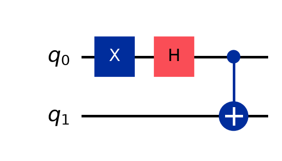
The 4 Bell states form an orthonormal basis for the entire two-qubit Hilbert space $\mathbb{C}^4$, known as the Bell basis. Any two-qubit state can be written as a linear combination of these four states:

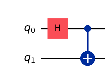
1. State $|\Phi^+\rangle = \frac{|00\rangle + |11\rangle}{\sqrt{2}}$ (Correlated, Positive Phase)

Prepared from $|00\rangle$ via $H(q_0)$ followed by $CX(q_0, q_1)$:

Circuit” style=”max-width:100%;height:auto;display:inline-block;border-radius:4px”>

Circuit 1: Preparation of |Phi+> from ground state |00>.

2. State $|\Phi^-\rangle = \frac{|00\rangle – |11\rangle}{\sqrt{2}}$ (Correlated, Negative Phase)

Prepared by applying an $X$ gate (or $Z$ gate) to $q_0$ before the Hadamard, creating $|-\rangle \otimes |0\rangle$ before the CNOT:

Circuit” style=”max-width:100%;height:auto;display:inline-block;border-radius:4px”>

Circuit 2: Preparation of |Phi-> with relative minus phase.

3. State $|\Psi^+\rangle = \frac{|01\rangle + |10\rangle}{\sqrt{2}}$ (Anti-Correlated, Positive Phase)

Prepared by flipping the target qubit $q_1$ with an $X$ gate, so the CNOT flips $|01\rangle \leftrightarrow |10\rangle$:

Circuit” style=”max-width:100%;height:auto;display:inline-block;border-radius:4px”>

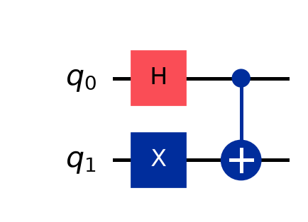
Circuit 3: Preparation of |Psi+> with bit-flip anti-correlation.

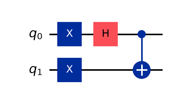
4. State $|\Psi^-\rangle = \frac{|01\rangle – |10\rangle}{\sqrt{2}}$ (The Singlet State)

Prepared with $X$ gates on both qubits before the entangling layer. $|\Psi^-\rangle$ is the unique anti-symmetric singlet state with total spin $S=0$, making it invariant under arbitrary simultaneous bilateral rotations:

Singlet Circuit” style=”max-width:100%;height:auto;display:inline-block;border-radius:4px”>

Circuit 4: Preparation of the rotationally invariant Singlet State |Psi->.

Bell Basis Properties Matrix

In our guide to the Bloch Sphere, we saw that any valid single-qubit pure state has a Bloch vector of length exactly $|\vec{r}| = 1$, residing on the outer spherical surface. What happens to the Bloch vector of qubit $A$ when it is entangled in $|\Phi^+\rangle$?

Because the composite state cannot be factored, we must represent qubit $A$’s state using a reduced density matrix $\rho_A$ by performing a partial trace over qubit $B$:

The Bloch vector coordinates are calculated from the Pauli expectations $r_i = \text{Tr}(\rho_A \sigma_i)$:

The Bloch vector vanishes completely into the exact center of the sphere! Qubit $A$ is in a maximally mixed state with purity $\text{Tr}(\rho_A^2) = 0.5$. Isolated from qubit $B$, qubit $A$ carries zero deterministic information—measuring it yields 50/50 pure random noise. Yet, the instant qubit $B$ is measured, the joint two-qubit correlation is 100% deterministic.

If we measure $|\Phi^+\rangle$ and $|\Phi^-\rangle$ directly in the computational basis, both produce `00` (50%) and `11` (50%). How can an experimenter distinguish all four Bell states deterministically?

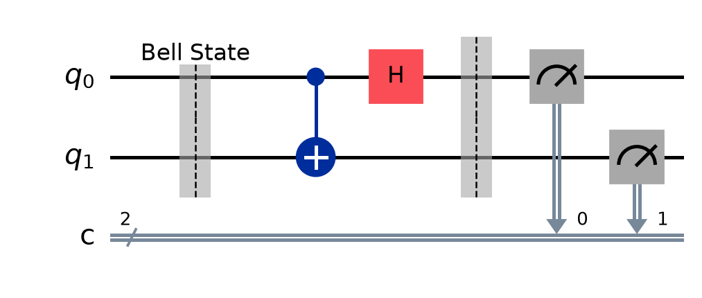
Because quantum circuits are unitary and reversible, we apply the inverse of the Bell preparation circuit: a CNOT gate followed by a Hadamard on the control qubit ($CX \to H$):

Circuit 5: The Bell Basis Decoder (CX followed by H) rotates the 4 entangled states back to the computational basis.

This transformation maps the 4 entangled Bell states back into the 4 classical basis bitstrings with 100% deterministic certainty:

• |Φ+⟩ ⟶ 00 (100%)
• |Φ−⟩ ⟶ 01 (100%)
• |Ψ+⟩ ⟶ 10 (100%)
• |Ψ−⟩ ⟶ 11 (100%)

This decoder is the foundational building block for Superdense Coding (transmitting 2 classical bits using only 1 physical qubit) and the receiver measurement in Quantum Teleportation.

The script below creates all 4 Bell states, evaluates their computational basis correlations, executes the Bell basis decoder, and computes the reduced density matrix purity using Qiskit 2.x primitives:

import numpy as np
from qiskit import QuantumCircuit
from qiskit.primitives import StatevectorSampler
from qiskit.quantum_info import Statevector, partial_trace, DensityMatrix

def build_bell_state(state_name: str) -> QuantumCircuit:
    """Builds a 2-qubit circuit preparing the requested Bell state."""
    qc = QuantumCircuit(2, 2)
    if state_name == "Phi+":
        qc.h(0)
        qc.cx(0, 1)
    elif state_name == "Phi-":
        qc.x(0)
        qc.h(0)
        qc.cx(0, 1)
    elif state_name == "Psi+":
        qc.h(0)
        qc.x(1)
        qc.cx(0, 1)
    elif state_name == "Psi-":
        qc.x(0)
        qc.h(0)
        qc.x(1)
        qc.cx(0, 1)
    else:
        raise ValueError(f"Unknown Bell state: {state_name}")
    return qc

sampler = StatevectorSampler()
bell_states = ["Phi+", "Phi-", "Psi+", "Psi-"]

print("=== 4 Bell States Generation & Verification ===")
for name in bell_states:
    qc = build_bell_state(name)
    sv = Statevector(qc)
    
    # 1. Measure in standard computational basis
    qc_comp = qc.copy()
    qc_comp.measure([0, 1], [0, 1])
    counts_comp = sampler.run([qc_comp], shots=1000).result()[0].data.c.get_counts()
    
    # 2. Decode back via Bell Basis Analyzer (CX then H)
    qc_decode = qc.copy()
    qc_decode.cx(0, 1)
    qc_decode.h(0)
    qc_decode.measure([0, 1], [0, 1])
    counts_dec = sampler.run([qc_decode], shots=100).result()[0].data.c.get_counts()
    
    print(f"State |{name}>:")
    print(f"  Statevector: {np.round(sv.data, 3)}")
    print(f"  Computational Basis (1000 shots): {counts_comp}")
    print(f"  Bell Basis Decoder (100 shots):    {counts_dec}\n")

# 3. Mathematical proof of Bloch sphere collapse: Partial Trace
phi_plus_sv = Statevector(build_bell_state("Phi+"))
rho_total = DensityMatrix(phi_plus_sv)
rho_A = partial_trace(rho_total, [1])  # trace out qubit B

print("Reduced Density Matrix of Qubit A:")
print(rho_A.data)
purity = np.real(np.trace(rho_A.data @ rho_A.data))
print(f"Purity Tr(rho_A^2): {purity:.2f} (0.50 = Maximally Mixed, Bloch radius r = 0)")

Execution Output:

=== 4 Bell States Generation & Verification ===
State |Phi+>:
  Statevector: [0.707+0.j 0.   +0.j 0.   +0.j 0.707+0.j]
  Computational Basis (1000 shots): {'00': 507, '11': 493}
  Bell Basis Decoder (100 shots):    {'00': 100}

State |Phi->:
  Statevector: [ 0.707+0.j  0.   +0.j  0.   +0.j -0.707+0.j]
  Computational Basis (1000 shots): {'00': 511, '11': 489}
  Bell Basis Decoder (100 shots):    {'01': 100}

State |Psi+>:
  Statevector: [0.   +0.j 0.707+0.j 0.707+0.j 0.   +0.j]
  Computational Basis (1000 shots): {'01': 476, '10': 524}
  Bell Basis Decoder (100 shots):    {'10': 100}

State |Psi->:
  Statevector: [ 0.   +0.j -0.707+0.j  0.707+0.j  0.   +0.j]
  Computational Basis (1000 shots): {'01': 501, '10': 499}
  Bell Basis Decoder (100 shots):    {'11': 100}

Reduced Density Matrix of Qubit A:
[[0.5+0.j 0. +0.j]
 [0. +0.j 0.5+0.j]]
Purity Tr(rho_A^2): 0.50 (0.50 = Maximally Mixed, Bloch radius r = 0)