Quantum Computing: The Deutsch-Jozsa Algorithm Explained — Classical vs. Quantum Complexity and Qiskit Implementation

We are given a black-box oracle that computes an unknown Boolean function taking an $n$-bit string and returning a single bit:

We are promised that $f$ belongs strictly to one of two categories:

• Constant: The function returns the exact same value for all possible inputs ($f(x) = 0$ for all $x$, or $f(x) = 1$ for all $x$).
• Balanced: The function returns 0 for exactly half of the $2^n$ inputs ($2^{n-1}$ states) and 1 for the remaining half ($2^{n-1}$ states).

The Objective: Determine with 100% mathematical certainty whether $f$ is constant or balanced using the absolute minimum number of oracle evaluations.

Classically, if you query the oracle with an input $x_1$ and receive $f(x_1) = 0$, you learn nothing definitive. If your next query $x_2$ yields $f(x_2) = 1$, you immediately know $f$ is balanced (best-case: 2 queries). However, in the worst-case scenario, every input you test continues to return 0.

Because a balanced function has exactly $2^{n-1}$ zeros, observing $2^{n-1}$ zeros in a row still leaves the possibility that the remaining $2^{n-1}$ inputs are all ones (balanced) or all zeros (constant). To be 100% deterministic, a classical computer must evaluate:

Quantum computing solves this in exactly 1 query ($O(1)$) with 100% certainty:

Note on randomized algorithms: A classical probabilistic algorithm could query $k$ random inputs; if all return 0, the chance of being wrong is $(1/2)^{k-1}$. While randomized testing is fast, only the quantum algorithm offers deterministic, exact certainty in $O(1)$.

To compute $f(x)$ reversibly, quantum computers use a unitary oracle $U_f$ operating on an input register $|x\rangle$ and an auxiliary target qubit $|y\rangle$:

Rather than preparing the target qubit in $|0\rangle$, we prepare it in the anti-symmetric superposition state $|-\rangle = \frac{|0\rangle – |1\rangle}{\sqrt{2}}$ using an $X$ gate followed by a Hadamard $H$. Watch what happens when $U_f$ evaluates:

In both cases, we can write the result compactly:

The bit $f(x)$ is not written to the target qubit at all—it is kicked back as an eigenvalue phase factor $(-1)^{f(x)}$ directly onto the input register state!

To understand how oracles are physically constructed, let us take a 3-qubit input register ($q_0, q_1, q_2$) with an auxiliary target qubit ($q_3$). Any Boolean function falls into one of four canonical implementations:

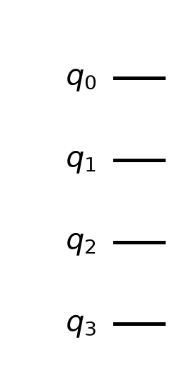
Oracle 1: Constant-0 ($f(x) = 0$ everywhere)

Because $y \oplus 0 = y$, the target qubit is left completely untouched. The circuit is an empty identity wire:

Oracle 1: Identity wire — target qubit q3 remains unchanged.

Oracle 2: Constant-1 ($f(x) = 1$ everywhere)

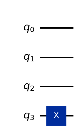
Because $y \oplus 1 = \bar{y}$, the target qubit must flip unconditionally for all inputs. We apply a single NOT ($X$) gate to $q_3$:

Oracle 2: Unconditional X gate on q3 — imparts an unobservable global minus sign.

Oracle 3: Balanced Direct ($f(x) = x_0 \oplus x_2$)

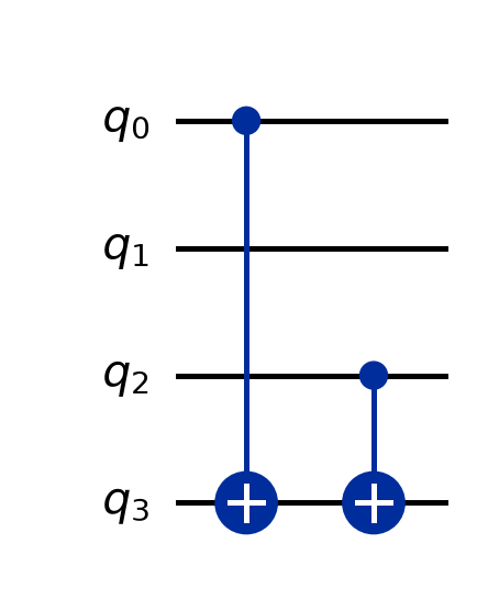
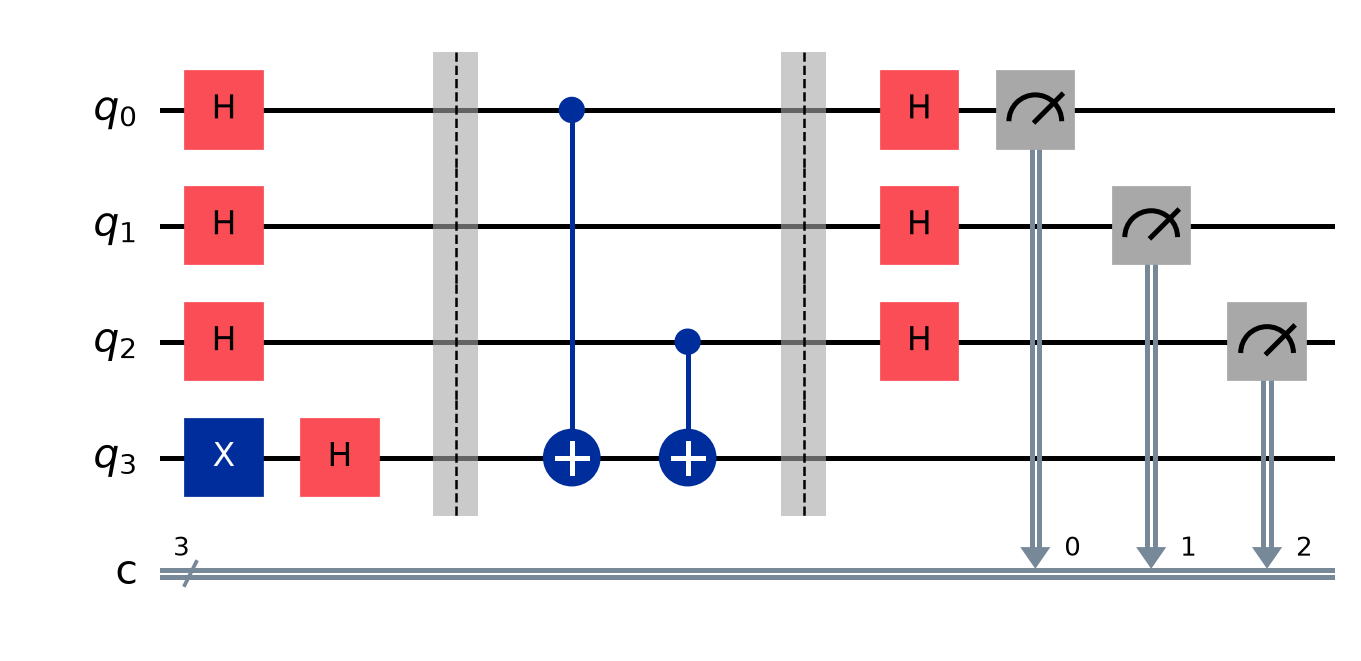
To create a balanced function, we can compute an inner product or parity check. In this example, CNOTs are placed on $q_0$ and $q_2$ targeting $q_3$, leaving $q_1$ unattached:

Oracle 3: CNOT controls on q0 and q2 — evaluates f(x) = x0 ⊕ x2.

Why does skipping $q_1$ still yield a balanced function? Because the function output is determined strictly by $x_0 \oplus x_2$. Across the 8 possible states, exactly 4 combinations give 0 (000, 010, 101, 111) and exactly 4 give 1 (001, 011, 100, 110). A balanced function does not need to depend on every qubit—it only needs an exact 50/50 output split across the $2^n$ state space.

Oracle 4: Balanced Inverted ($f(x) = \neg(x_0 \oplus x_2) = x_0 \oplus x_2 \oplus 1$)

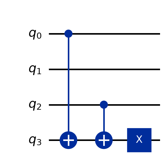
This is the complement of Oracle 3 (inverting all outputs). We place CNOTs on $q_0$ and $q_2$, followed by an $X$ gate on target $q_3$:

Oracle 4: CNOT controls on q0 and q2 followed by NOT on q3.

Oracle Comparison Matrix

Here is the complete end-to-end Deutsch-Jozsa circuit for our 3-qubit balanced function ($f(x) = x_0 \oplus x_2$):

Complete Deutsch-Jozsa Circuit in Qiskit (IBM Quantum styling): State prep, superposition, oracle, interference Hadamards, and measurement.

The Mathematical Interference:

Before the final Hadamard transform, the input register is in the state $\frac{1}{\sqrt{2^n}} \sum_{x} (-1)^{f(x)} |x\rangle$. Applying the Walsh-Hadamard transform $H^{\otimes n}$ maps each basis state $|x\rangle$ to $\frac{1}{\sqrt{2^n}} \sum_{z} (-1)^{x \cdot z} |z\rangle$. The total state becomes:

When we measure, consider the probability amplitude of measuring the all-zero state $|00\dots 0\rangle$ (where $z = 00\dots 0 \implies x \cdot z = 0$):

• If $f$ is Constant: All $(-1)^{f(x)}$ have the same sign ($\pm 1$). The sum adds constructively: $\alpha_{00\dots 0} = \frac{1}{2^n} (\pm 2^n) = \pm 1$. The measurement probability is $|\pm 1|^2 = \mathbf{100\%}$. You will measure `00…0` every single time.
• If $f$ is Balanced: Exactly $2^{n-1}$ inputs yield $+1$ and $2^{n-1}$ yield $-1$. The sum cancels out completely: $\alpha_{00\dots 0} = \frac{1}{2^n} (2^{n-1} – 2^{n-1}) = \mathbf{0}$. The probability of measuring all zeros is strictly 0%! Any non-zero bitstring confirms $f$ is balanced.

The script below builds, executes, and verifies all 4 oracles using modern Qiskit 2.x primitives (StatevectorSampler):

from qiskit import QuantumCircuit
from qiskit.primitives import StatevectorSampler

def create_oracle(oracle_type: str) -> QuantumCircuit:
    """Builds one of the 4 canonical oracles on 4 qubits (q0, q1, q2 input; q3 target)."""
    oracle = QuantumCircuit(4, name=oracle_type)
    
    if oracle_type == "constant_0":
        # Type 1: f(x) = 0 (Identity wire)
        pass
    elif oracle_type == "constant_1":
        # Type 2: f(x) = 1 (Unconditional target flip)
        oracle.x(3)
    elif oracle_type == "balanced_direct":
        # Type 3: f(x) = x0 ^ x2 (CNOT parity on q0 and q2)
        oracle.cx(0, 3)
        oracle.cx(2, 3)
    elif oracle_type == "balanced_inverted":
        # Type 4: f(x) = ~(x0 ^ x2) (CNOT parity + NOT gate)
        oracle.cx(0, 3)
        oracle.cx(2, 3)
        oracle.x(3)
    else:
        raise ValueError(f"Unknown oracle type: {oracle_type}")
        
    return oracle

def run_deutsch_jozsa(oracle_circuit: QuantumCircuit):
    """Wraps an oracle inside the full Deutsch-Jozsa algorithm and measures."""
    qc = QuantumCircuit(4, 3)
    
    # 1. State preparation: target qubit to |->
    qc.x(3)
    qc.h(range(4))
    qc.barrier()
    
    # 2. Insert the oracle
    qc.compose(oracle_circuit, inplace=True)
    qc.barrier()
    
    # 3. Interference decoding
    qc.h(range(3))
    
    # 4. Measure input register
    qc.measure([0, 1, 2], [0, 1, 2])
    
    # Execute on StatevectorSampler
    sampler = StatevectorSampler()
    result = sampler.run([qc], shots=100).result()
    counts = result[0].data.c.get_counts()
    verdict = "CONSTANT" if list(counts.keys()) == ['000'] else "BALANCED"
    
    return qc, counts, verdict

# Execute and compare all 4 canonical oracles
oracles = ["constant_0", "constant_1", "balanced_direct", "balanced_inverted"]

print(f"{'Oracle Type':<20} | {'Measurement':<12} | {'Decision':<10}")
print("-" * 50)
for o_name in oracles:
    oracle_qc = create_oracle(o_name)
    full_qc, counts, verdict = run_deutsch_jozsa(oracle_qc)
    print(f"{o_name:<20} | {str(counts):<12} | {verdict:<10}")

Execution Output:

Oracle Type          | Measurement  | Decision  
--------------------------------------------------
constant_0           | {'000': 100} | CONSTANT  
constant_1           | {'000': 100} | CONSTANT  
balanced_direct      | {'101': 100} | BALANCED  
balanced_inverted    | {'101': 100} | BALANCED