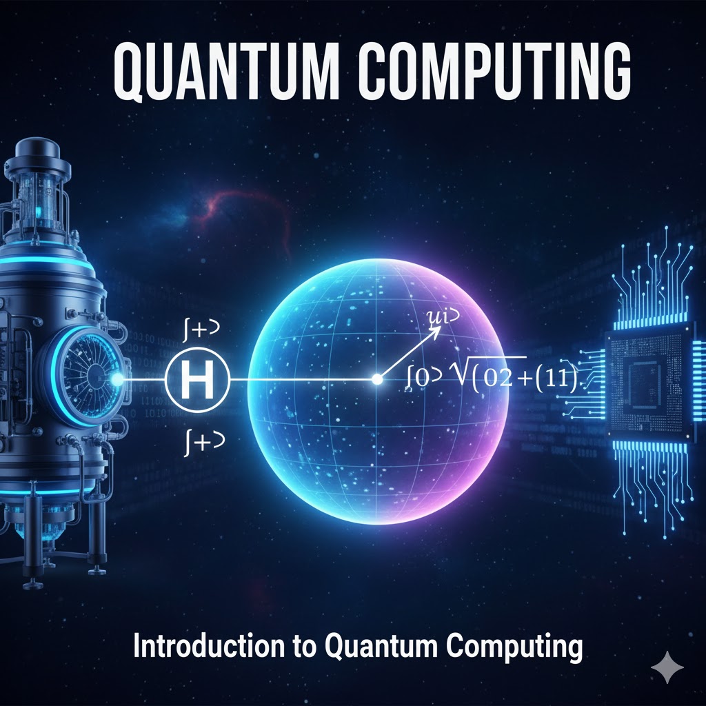
Qubits, the Hadamard gate, superposition, tensor products, and quantum interference from first principles.
Classical computers store information in bits that are always exactly 0 or 1. Quantum computers exploit the principles of quantum mechanics to do something fundamentally different: they operate on qubits, which can exist in a superposition of both states simultaneously. The Hadamard gate is the simplest gate that creates this superposition, and understanding it from first principles is the entry point to every quantum algorithm that follows.
1 · The Qubit
A qubit is the fundamental unit of quantum information. Unlike a classical bit, a qubit can exist in a superposition of |0⟩ and |1⟩ simultaneously. We write its general state using Dirac (bra-ket) notation:
Here α and β are complex numbers called probability amplitudes. They must satisfy the normalisation condition:
The two computational basis states are represented as column vectors:
0
1
When we measure the qubit in state |ψ⟩ = α|0⟩ + β|1⟩, we get |0⟩ with probability |α|² and |1⟩ with probability |β|². The act of measurement destroys the superposition and collapses the qubit to a definite classical state.
2 · The Hadamard Gate
The Hadamard gate H is a 2×2 unitary matrix that maps each computational basis state to an equal superposition:
+1 −1
Applying H to each basis state:
| Input | H |input⟩ | Short name |
|---|---|---|
| |0⟩ | (1/√2)( |0⟩ + |1⟩ ) | |+⟩ |
| |1⟩ | (1/√2)( |0⟩ − |1⟩ ) | |−⟩ |
Both outputs have equal amplitudes of 1/√2, giving a 50% measurement probability for each outcome. The sign difference between |+⟩ and |−⟩ is what drives interference later.
3 · H² = I: Quantum Interference
Applying H twice to |0⟩ returns the qubit to |0⟩. The algebra shows exactly why the |1⟩ amplitudes cancel through destructive interference:
= H( (1/√2)(|0⟩ + |1⟩) )
= (1/√2)( H|0⟩ + H|1⟩ )
= (1/√2)( (1/√2)(|0⟩+|1⟩) + (1/√2)(|0⟩−|1⟩) )
= (1/2)( |0⟩ + |1⟩ + |0⟩ − |1⟩ )
= (1/2)( 2|0⟩ )
= |0⟩ ✓
4 · Single-Qubit Circuit: H–H–Measure
A single qubit routed through two Hadamard gates and then measured always returns 0 with 100% probability:
| Step | State | Notes |
|---|---|---|
| 1. Initialise | |ψ₀⟩ = |0⟩ | Ground state |
| 2. First H | |ψ₁⟩ = (1/√2)(|0⟩+|1⟩) | Superposition: 50/50 |
| 3. Second H | |ψ₂⟩ = |0⟩ | Interference collapses back |
| 4. Measure | Result = 0 | 100% probability |
5 · Tensor Products and Multi-Qubit States
Multi-qubit systems are described using the tensor product (⊗). For two qubits, the four computational basis states are:
| Ket | Tensor form | Column vector |
|---|---|---|
| |00⟩ | |0⟩ ⊗ |0⟩ | [1, 0, 0, 0]ᵀ |
| |01⟩ | |0⟩ ⊗ |1⟩ | [0, 1, 0, 0]ᵀ |
| |10⟩ | |1⟩ ⊗ |0⟩ | [0, 0, 1, 0]ᵀ |
| |11⟩ | |1⟩ ⊗ |1⟩ | [0, 0, 0, 1]ᵀ |
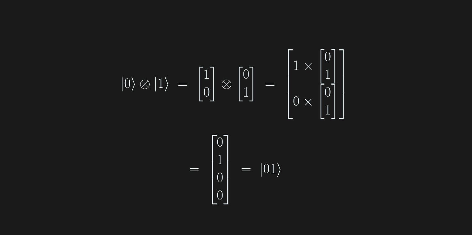
The tensor product of two vectors is computed by multiplying each element of the first vector by the entire second vector and stacking the results. For |0⟩ ⊗ |1⟩:
6 · Two-Qubit Superposition: H⊗H on |00⟩
Applying independent Hadamard gates to both qubits starting from |00⟩:
= (H|0⟩) ⊗ (H|0⟩)
= (1/√2)(|0⟩+|1⟩) ⊗ (1/√2)(|0⟩+|1⟩)
= (1/2)( |00⟩ + |01⟩ + |10⟩ + |11⟩ )
7 · Interference in a Two-Qubit H–H Circuit
Applying H⊗H twice to |00⟩ returns it to |00⟩. The interference analysis on each basis state shows the mechanism:
| Input to 2nd H⊗H | After (H⊗H) |
|---|---|
| |00⟩ | (1/2)( |00⟩ + |01⟩ + |10⟩ + |11⟩ ) |
| |01⟩ | (1/2)( |00⟩ − |01⟩ + |10⟩ − |11⟩ ) |
| |10⟩ | (1/2)( |00⟩ + |01⟩ − |10⟩ − |11⟩ ) |
| |11⟩ | (1/2)( |00⟩ − |01⟩ − |10⟩ + |11⟩ ) |
The initial superposition has equal weight 1/2 on each of the four states. Summing contributions to each output:
| Output state | Amplitude sum (× 1/4) | Result |
|---|---|---|
| |00⟩ | +1 +1 +1 +1 | 4/4 = 1 ✓ constructive |
| |01⟩ | +1 −1 +1 −1 | 0 destructive |
| |10⟩ | +1 +1 −1 −1 | 0 destructive |
| |11⟩ | +1 −1 −1 +1 | 0 destructive |
8 · The H⊗H Matrix and Why It Matters
The combined H⊗H operator is a 4×4 Walsh-Hadamard matrix (scaled by 1/2). Its sign pattern is exactly the two-qubit case of the popcount rule derived in the Walsh-Hadamard post:
+1 −1 +1 −1
+1 +1 −1 −1
+1 −1 −1 +1
Every quantum algorithm that achieves a speedup over classical computation does so through the same three-phase structure:
| Phase | Operation | Purpose |
|---|---|---|
| 1. Open | Hadamard on all qubits | Create uniform superposition over all 2ⁿ states |
| 2. Operate | Oracle / phase manipulation | Mark or bias the amplitude of the target answer |
| 3. Close | Hadamard again (+ measurement) | Interference concentrates probability on the answer |
Hadamard tensor powers: H², H ⊗ H, and H⊗n
Why does H² = I?
The Hadamard matrix is H = (1/√2)[[1, 1], [1, −1]]. Multiplying it by itself gives:
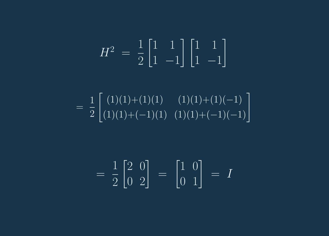
The first H changes the computational basis into the |+⟩ and |−⟩ basis. The second H changes it back. In amplitude terms, the unwanted paths cancel through destructive interference while the original basis-state amplitude adds constructively. Therefore H is its own inverse: applying it twice restores any one-qubit state.
Two qubits: H ⊗ H
Applying H independently to two qubits is written H ⊗ H = H⊗2. In the basis order |00⟩, |01⟩, |10⟩, |11⟩, its matrix is:
[[ 1,   1,   1,   1],
 [ 1,  −1,   1,  −1],
 [ 1,   1,  −1,  −1],
 [ 1,  −1,  −1,   1]]
For example, (H ⊗ H)|00⟩ = (|00⟩ + |01⟩ + |10⟩ + |11⟩)/2. Each basis state has amplitude 1/2 and probability 1/4.
Three qubits: H⊗3
For three qubits the operator is an 8 × 8 matrix. Using basis order |000⟩ through |111⟩:
[[ 1,   1,   1,   1,   1,   1,   1,   1],
 [ 1,  −1,   1,  −1,   1,  −1,   1,  −1],
 [ 1,   1,  −1,  −1,   1,   1,  −1,  −1],
 [ 1,  −1,  −1,   1,   1,  −1,  −1,   1],
 [ 1,   1,   1,   1,  −1,  −1,  −1,  −1],
 [ 1,  −1,   1,  −1,  −1,   1,  −1,   1],
 [ 1,   1,  −1,  −1,  −1,  −1,   1,   1],
 [ 1,  −1,  −1,   1,  −1,   1,   1,  −1]]
Applied to |000⟩, this produces all eight three-qubit basis states with amplitude 1/√8 and probability 1/8 each.
The general n-qubit rule
Applying H to every qubit is written H⊗n. It acts on a computational basis state |x⟩ as:
The binary inner product x·y determines each plus or minus sign. For x = 0…0, every sign is positive, giving a uniform superposition over all 2n basis states. Independent Hadamard gates do not create entanglement by themselves; an interaction such as a controlled-NOT gate is needed.
Small Qiskit example
This Qiskit example creates the three-qubit uniform superposition, confirms that every outcome has probability 1/8, and then applies H to all three qubits again to recover |000⟩.
from qiskit import QuantumCircuit
from qiskit.quantum_info import Statevector

qc = QuantumCircuit(3)
qc.h(range(3))

uniform = Statevector.from_instruction(qc)
print(uniform.probabilities_dict())
# 000 through 111 each have probability 0.125

qc.h(range(3))
restored = Statevector.from_instruction(qc)
print(restored.probabilities_dict())
# {'000': 1.0}Malcolm Low is an Associate Professor at the Singapore Institute of Technology, writing on quantum computing, programming, and applied computing from Singapore.
Website: malcolmlow.com · Singapore
Quantum Series 2026 · Built with Qiskit 1.x
✦ This article was generated with the assistance of Claude by Anthropic ✦
Share this:
- Share on Facebook (Opens in new window) Facebook
- Email a link to a friend (Opens in new window) Email
- Share on LinkedIn (Opens in new window) LinkedIn
- Share on Telegram (Opens in new window) Telegram
- Share on WhatsApp (Opens in new window) WhatsApp
- More
- Share on Bluesky (Opens in new window) Bluesky
- Print (Opens in new window) Print
- Share on Threads (Opens in new window) Threads
- Share on Reddit (Opens in new window) Reddit
- Share on Tumblr (Opens in new window) Tumblr
- Share on Pinterest (Opens in new window) Pinterest
- Share on X (Opens in new window) X


Leave a comment