How to Solve Quadratic Equations: The Po-Shen Loh Method
For four millennia—spanning Babylonian clay tablets, Renaissance cryptanalysts, and modern classrooms—solving quadratic equations has represented humanity’s gateway to abstract algebra. Yet standard pedagogy traps learners in a frustrating compromise between trial-and-error factoring and rote memorization of the quadratic formula. In late 2019, Carnegie Mellon professor and USA Math Olympiad head coach Po-Shen Loh unveiled an alternative derivation that bridges geometric parabola symmetry with 16th-century root relations.
By decomposing the problem into finding the parabolic axis of symmetry and computing a symmetric root offset via an elementary difference of squares, the Po-Shen Loh method renders quadratic equations solvable from first principles without guesswork, completing-the-square algebra tricks, or black-box formulas. In this comprehensive guide, we unpack the mathematical mechanics of the algorithm, explore its Renaissance origins under French royal cryptanalyst François Viète, visualize all three geometric root regimes with standalone graphs, analyze worked numerical examples across real, irrational, and complex roots, and benchmark its implications for floating-point numerical computing with complete Python verification code.
For thousands of years—dating back to the Old Babylonian Empire around 2000 BCE—mathematicians and students have tackled quadratic equations. Yet in standard high-school algebra curriculums worldwide, solving a quadratic equation such as x2 + Bx + C = 0 remains one of the most error-prone milestones for learners. The traditional curriculum forces students into a false binary between two deeply flawed approaches:
-
Guess-and-Check Factoring: Students are instructed to search by mental trial-and-error for two numbers that multiply to
Cand sum toB. While manageable for trivial textbook integers likex2 − 5x + 6 = 0, this strategy completely breaks down whenever coefficients are large, fractional, irrational, or complex. -
Blind Formula Memorization: When factoring fails, students are made to recite the quadratic formula by rote:
x = (−b ± √(b2 − 4ac)) / (2a). Divorced from geometric intuition, students regularly make sign errors when computing the discriminantb2 − 4ac, misapply the double negative on−b, or omit dividing by2a.
In December 2019, Professor Po-Shen Loh, a professor of mathematics at Carnegie Mellon University and longtime national coach of the USA International Mathematical Olympiad (IMO) team, published a paper titled A Simple Proof of the Quadratic Formula. He illuminated a remarkable pedagogical oversight: an intuitive, symmetry-first technique that solves any quadratic equation without guesswork, without completing the square tricks, and without memorizing the quadratic formula.
To understand how Po-Shen Loh’s method works, one must first meet the towering Renaissance thinker whose formulas made it possible: François Viète (1540–1603), commonly known by his Latinized name Franciscus Vieta.
Viète was not an academic mathematician by profession; he was a distinguished French lawyer and royal privy councillor serving King Henry III and King Henry IV of France during the turbulent French Wars of Religion. In addition to high statecraft, Viète was an extraordinary cryptanalyst. During the war against Spain, King Philip II of Spain utilized an ultra-secure code comprising over 500 secret symbols. Viète cracked the Spanish cipher completely, allowing the French Crown to intercept and decode Spanish military dispatches in real time. The Spanish crown was so mystified by France’s uncanny foresight that King Philip II complained to Pope Clement VIII, claiming that Viète was a sorcerer employing the black arts of divination!
In mathematics, Viète earned historical immortality as the “Father of Modern Algebraic Notation”. Prior to Viète, algebra was rhetorical—mathematicians described equations in long, verbose conversational sentences. In his 1591 masterpiece In artem analyticem isagoge (“Introduction to the Analytic Art”), Viète introduced the revolutionary concept of using letters systematically to represent both unknowns and known parameters.
Most crucially, Viète discovered the universal relations that now bear his name: Vieta’s Formulas. Viète observed that any polynomial can be factored directly through its roots:
(x − r1)(x − r2) = x2 − (r1 + r2)x + r1r2 = 0
Equating this expansion to the monic quadratic equation x2 + Bx + C = 0 reveals the fundamental connection:
-
Sum of roots:
r1 + r2 = −B -
Product of roots:
r1 · r2 = C
Every standard quadratic equation x2 + Bx + C = 0 can be graphed as a parabola y = x2 + Bx + C. A foundational geometric property of parabolas is bilateral symmetry: the curve is mirrored across its vertical axis of symmetry. If the parabola intersects the horizontal axis at two roots, r1 and r2, those roots must be located at an equal distance from the axis of symmetry.
Because Vieta’s formula proves that the sum of the two roots is −B, their exact midpoint (the axis of symmetry) is simply their arithmetic mean:
m = (r1 + r2) / 2 = −B / 2
Since the two roots are symmetrically spaced around the midpoint m, we can represent them with an unknown offset u:
r1 = m − u = −B/2 − u
r2 = m + u = −B/2 + u
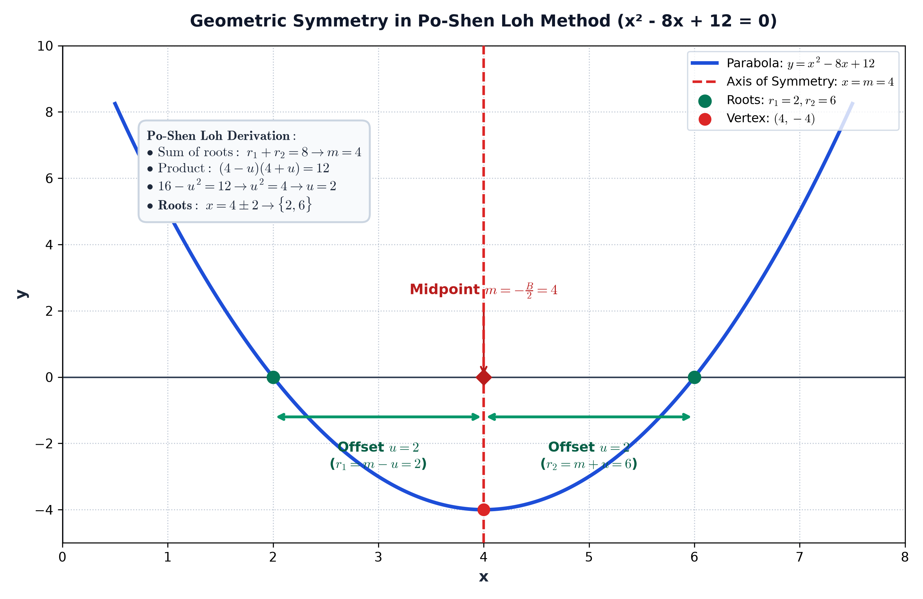
Figure 1: Geometric symmetry of the quadratic curve y = x2 − 8x + 12. The axis of symmetry sits at x = m = 4, and both roots r1 = 2 and r2 = 6 lie at an equal distance u = 2 from the midpoint.
Now comes the stroke of genius: Vieta’s second relation tells us that the product of the two roots must equal C. Substituting our symmetric expressions yields an elementary difference of squares:
(m − u)(m + u) = C
m2 − u2 = C
u2 = m2 − C
u = √(m2 − C)
u, the roots are immediately x = m ± u. There is no guessing, no trial factoring, and no cumbersome discriminant algebraic manipulation.
Whenever you encounter any quadratic equation, execute these three straightforward algorithmic steps:
-
Normalize to Monic Form: If the equation has a leading coefficient
ax2 + bx + c = 0witha ≠ 1, divide through byato obtainx2 + Bx + C = 0, whereB = b/aandC = c/a. -
Compute the Midpoint: Compute the midpoint
m = −B / 2. Express the two roots asm − uandm + u. -
Solve for the Offset
u: Setm2 − u2 = C, which yieldsu = √(m2 − C). The final roots arem − uandm + u.
b2 − 4ac and across the fraction bar simultaneously. In Po-Shen Loh’s algorithm, the midpoint sign is resolved in isolation at Step 2 (m = −B/2), while the offset step is a clean difference of squares (u2 = m2 − C).
In traditional algebra, students memorize the discriminant Δ = b2 − 4ac to test whether roots are real or complex. In Po-Shen Loh’s formulation, the exact same behavior is captured naturally by the sign of u2 = m2 − C across three distinct geometric configurations:
Case 1: Positive Offset (u2 > 0) — Two Distinct Real Roots
When m2 > C, the offset squared is strictly positive (u2 > 0). Geometrically, this means the vertex of the parabola dips below the horizontal axis. As a result, the curve cuts the axis at two separate real points: m − u and m + u.
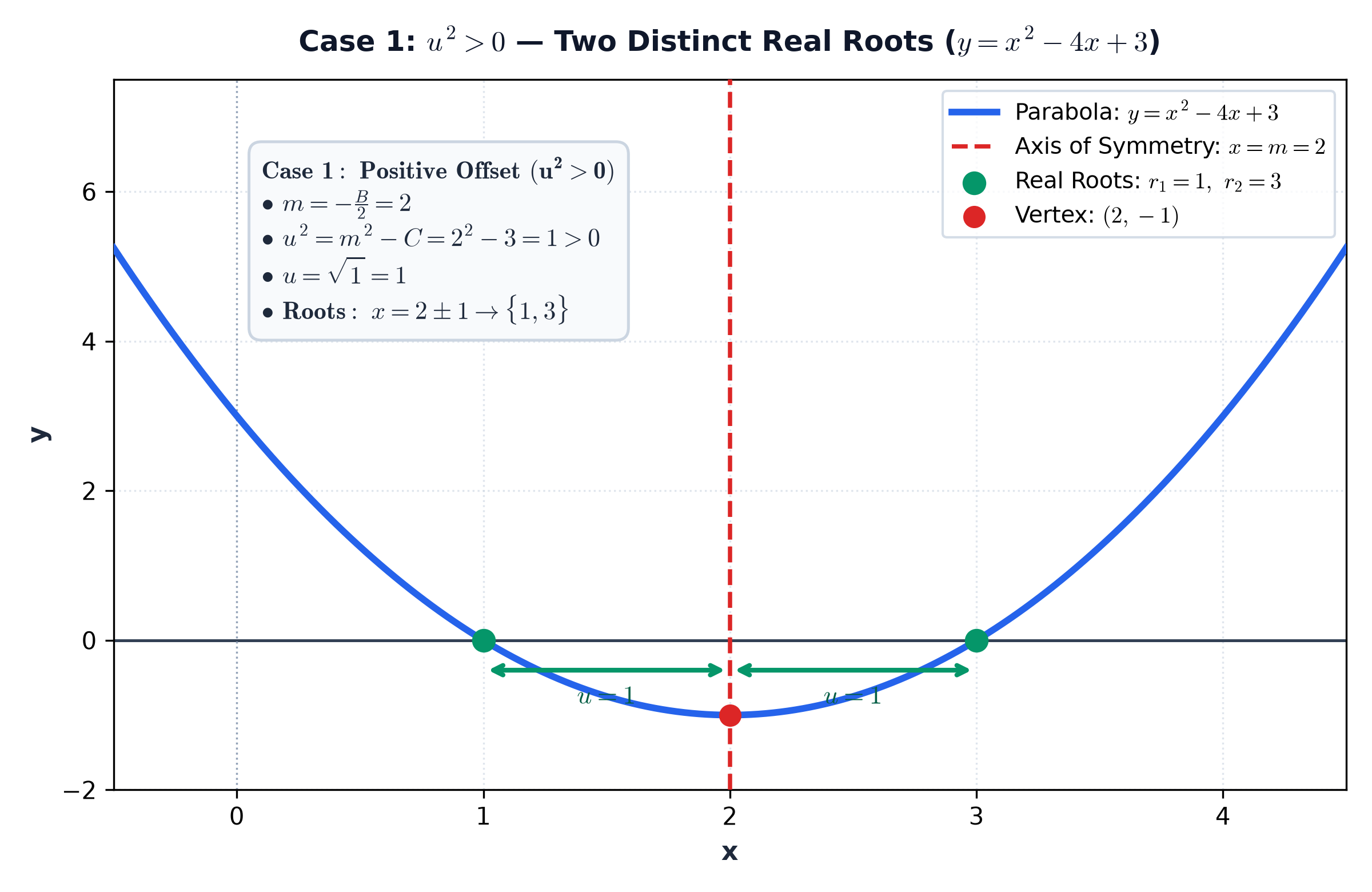
Figure 2: Case 1: Positive offset (u2 > 0). The parabola y = x2 − 4x + 3 dips below the horizontal axis, producing two distinct real roots at x = 2 − 1 = 1 and x = 2 + 1 = 3.
Case 2: Zero Offset (u2 = 0) — One Repeated Real Root
When m2 = C, the offset squared equals zero (u2 = 0). Geometrically, the vertex of the parabola touches the horizontal axis tangentially. The offset vanishes (u = 0), yielding a single repeated real root directly at the vertex coordinate x = m.
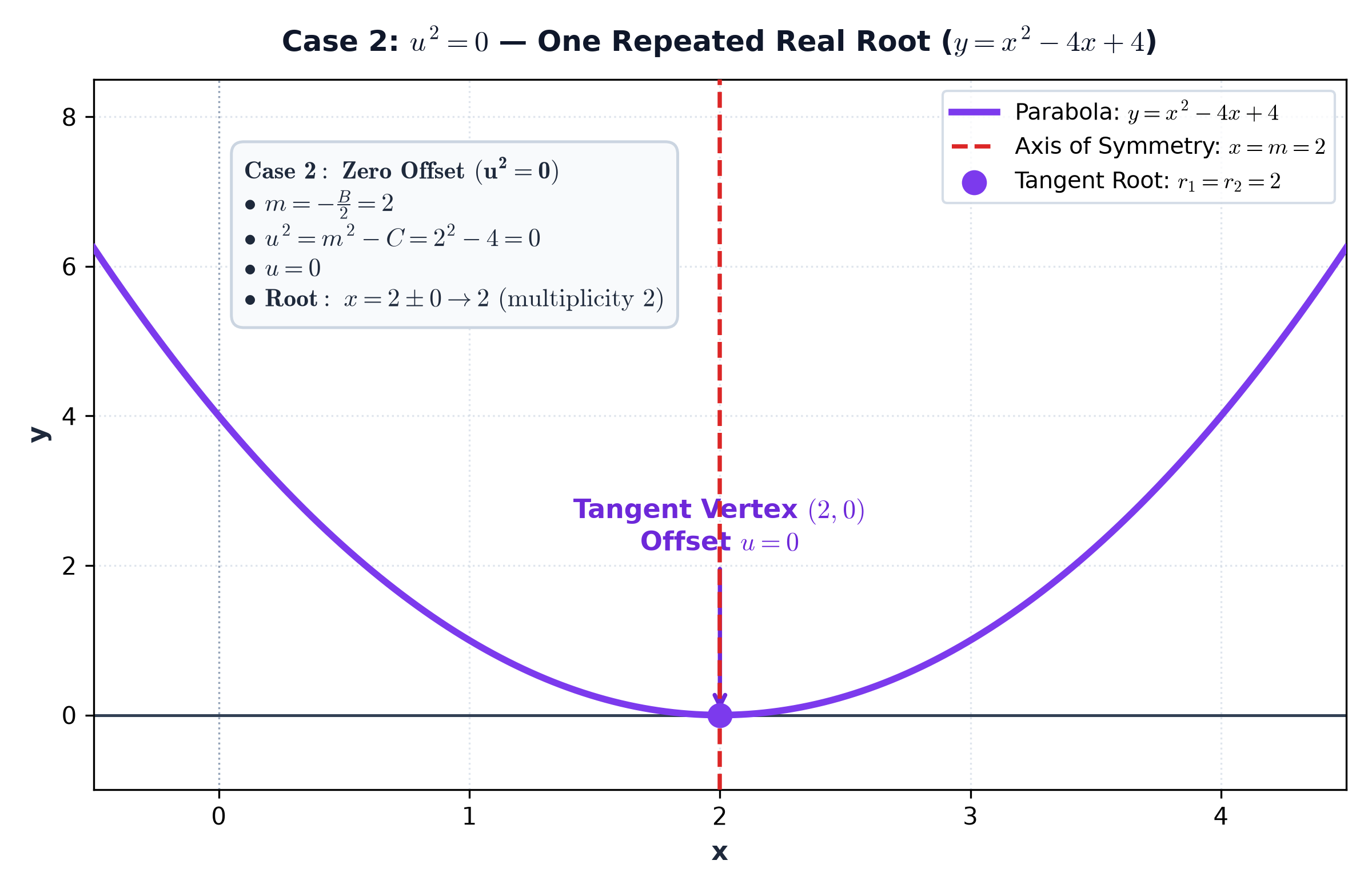
Figure 3: Case 2: Zero offset (u2 = 0). The vertex of y = x2 − 4x + 4 is tangent to the horizontal axis at (2, 0), producing a single repeated real root at x = 2.
Case 3: Negative Offset (u2 < 0) — Two Complex Conjugate Roots
When m2 < C, the offset squared is strictly negative (u2 < 0). Geometrically, the parabola floats completely above the horizontal axis and never intersects y = 0. Here u = i√(C − m2), immediately producing complex conjugate roots m ± iu without any separate case formulas or quadratic formula re-evaluations.
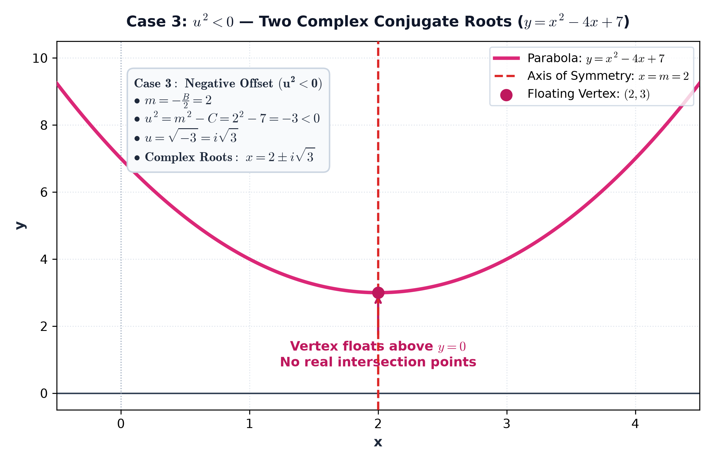
Figure 4: Case 3: Negative offset (u2 < 0). The parabola y = x2 − 4x + 7 floats entirely above the horizontal axis with its vertex at (2, 3), yielding two complex conjugate roots at x = 2 ± i√3.
Example 1: Standard Integer Roots (Eliminating Guesswork)
Solve the equation: x2 − 8x + 12 = 0.
Step 1 — Normalize & Identify Coefficients
The equation is monic with B = −8 and C = 12.
Step 2 — Compute Midpoint
Midpoint m = −(−8) / 2 = 4. The roots are 4 − u and 4 + u.
Step 3 — Difference of Squares Offset
42 − u2 = 12 → 16 − u2 = 12 → u2 = 4 → u = 2.
Roots: x = 4 − 2 = 2 and x = 4 + 2 = 6
Example 2: Irrational Roots (Where Factoring Completely Fails)
Solve the equation: x2 − 4x − 1 = 0.
Step 1 — Normalize & Identify Coefficients
Normalized with B = −4 and C = −1. Factoring is impossible because no rational factors of −1 sum to −4.
Step 2 — Compute Midpoint
Midpoint m = −(−4) / 2 = 2. Roots are 2 − u and 2 + u.
Step 3 — Difference of Squares Offset
22 − u2 = −1 → 4 − u2 = −1 → u2 = 5 → u = √5.
Roots: x = 2 − √5 and x = 2 + √5
Example 3: Complex / Imaginary Roots
Solve the equation: x2 − 6x + 25 = 0.
Step 1 — Normalize & Identify Coefficients
Normalized with B = −6 and C = 25.
Step 2 — Compute Midpoint
Midpoint m = −(−6) / 2 = 3. Roots are 3 − u and 3 + u.
Step 3 — Difference of Squares Offset
32 − u2 = 25 → 9 − u2 = 25 → u2 = −16 → u = 4i.
Roots: x = 3 − 4i and x = 3 + 4i
Example 4: Leading Coefficient a ≠ 1
Solve the equation: 2x2 + 5x − 3 = 0.
Step 1 — Normalize to Monic Form
Divide by 2: x2 + (5/2)x − 3/2 = 0. Here B = 5/2 and C = −3/2.
Step 2 — Compute Midpoint
Midpoint m = −(5/2) / 2 = −5/4. Roots are −5/4 − u and −5/4 + u.
Step 3 — Difference of Squares Offset
(−5/4)2 − u2 = −3/2 → 25/16 − u2 = −24/16 → u2 = 49/16 → u = 7/4.
Roots: x = −5/4 − 7/4 = −12/4 = −3 and x = −5/4 + 7/4 = 2/4 = 1/2
Below is a structured architectural comparison between traditional textbook quadratic methods and the Po-Shen Loh formulation:
↔ Scroll horizontally to view full comparison on mobile or smaller screens
| Feature | Traditional Quadratic Formula | Po-Shen Loh Method |
|---|---|---|
| Core Strategy | Rote substitution into cumbersome algebraic formula | Geometric symmetry around midpoint + difference of squares |
| Mental Complexity | High: multi-step numerator squaring and 4ac multiplication |
Minimal: simple single-step square m2 − C |
| Sign Error Rate | Frequent errors with negative b, negative c, and division |
Sign errors virtually eliminated due to isolated midpoint step |
| Pedagogical Value | Black-box memorization; zero geometric intuition | Directly connects Vieta’s formulas, parabolas, and algebra |
Beyond secondary education, Po-Shen Loh’s formulation holds important computational implications for numerical software, ray-tracing intersection algorithms, and physics simulation engines:
-
Catastrophic Floating-Point Cancellation: In IEEE 754 floating-point arithmetic, the traditional formula expression
−b + √(b2 − 4ac)loses catastrophic precision whenb2 ≫ 4acbecause two nearly identical large numbers are subtracted. Computing the midpointmand offsetuseparately provides an intuitive pathway to stable formulations such as Citardauq’s formula or Muller’s method. -
Ray-Sphere Collision Optimization: Decomposing the root calculation into finding the vertex coordinate
x = −B/2and testing whetherm2 ≥ Cmirrors how real-time rendering engines test bounding volume sphere intersections without computing square roots unless an actual surface penetration occurs.
Below is a clean, self-contained Python implementation of the Po-Shen Loh quadratic algorithm that supports integer, irrational, and complex roots:
import math

def solve_po_shen_loh(a: float, b: float, c: float):
    """
    Solves ax^2 + bx + c = 0 using the Po-Shen Loh method.
    Returns (r1, r2, regime)
    """
    if a == 0:
        raise ValueError("Leading coefficient 'a' cannot be zero.")

    # Step 1: Normalize to monic form x^2 + Bx + C = 0
    B = b / a
    C = c / a

    # Step 2: Compute midpoint m = -B / 2
    m = -B / 2.0

    # Step 3: Compute offset squared u^2 = m^2 - C
    u_squared = m**2 - C

    if abs(u_squared) < 1e-12:
        # Case 2: One repeated real root (u = 0)
        return (m, m, "Repeated Real Root")
    elif u_squared > 0:
        # Case 1: Two distinct real roots
        u = math.sqrt(u_squared)
        return (m - u, m + u, "Two Distinct Real Roots")
    else:
        # Case 3: Two complex conjugate roots
        u_imag = math.sqrt(-u_squared)
        return (complex(m, -u_imag), complex(m, u_imag), "Two Complex Conjugate Roots")

def format_root(r):
    if isinstance(r, complex):
        return f"{r.real:.1f}{r.imag:+.1f}j"
    return f"{r:.4f}"

# Run verification test cases
test_cases = [
    (1, -8, 12, "x^2 - 8x + 12 = 0"),
    (1, -4, -1, "x^2 - 4x - 1 = 0"),
    (1, -6, 25, "x^2 - 6x + 25 = 0"),
    (2,  5, -3, "2x^2 + 5x - 3 = 0"),
    (1, -4,  4, "x^2 - 4x + 4 = 0")
]

print("{:20} | {:15} | {:15} | {}".format("Equation", "Root 1", "Root 2", "Regime"))
print("-" * 75)
for a, b, c, label in test_cases:
    r1, r2, regime = solve_po_shen_loh(a, b, c)
    print("{:20} | {:15} | {:15} | {}".format(label, format_root(r1), format_root(r2), regime))
Verifiable Terminal Output:
Equation             | Root 1          | Root 2          | Regime
---------------------------------------------------------------------------
x^2 - 8x + 12 = 0    | 2.0000          | 6.0000          | Two Distinct Real Roots
x^2 - 4x - 1 = 0     | -0.2361         | 4.2361          | Two Distinct Real Roots
x^2 - 6x + 25 = 0    | 3.0-4.0j        | 3.0+4.0j        | Two Complex Conjugate Roots
2x^2 + 5x - 3 = 0    | -3.0000         | 0.5000          | Two Distinct Real Roots
x^2 - 4x + 4 = 0 | 2.0000 | 2.0000 | Repeated Real Root-
Symmetry Replaces Factoring: Instead of guessing factor pairs of
Cthat sum toB, the Po-Shen Loh method computes the exact midpointm = −B/2and finds the symmetric offset via difference of squaresu2 = m2 − C. - Vieta’s Formulas Form the Backbone: The method relies directly on 16th-century relations established by French royal cryptanalyst François Viète, proving that polynomial roots can be manipulated through their symmetric sum and product without pre-calculating values.
-
All Three Root Cases Unified: Whether roots are distinct real (
u2 > 0), repeated real (u2 = 0), or complex conjugate (u2 < 0), the exact same three algebraic steps apply without branching or separate formulas. -
Sign Errors Eliminated: Isolating the midpoint calculation
m = −B/2from the offset calculation eliminates the most common student pitfall in classical algebra: mishandling signs inside√(b2 − 4ac).
Does the Po-Shen Loh method replace the quadratic formula?
Mathematically, the Po-Shen Loh method is equivalent to the quadratic formula—in fact, writing out m = −b/(2a) and u = √((−b/(2a))2 − c/a) directly derives the standard formula. However, pedagogically and practically, it completely replaces the need to memorize the formula, enabling students and practitioners to derive roots intuitively from first principles.
Who was Vieta and what is his connection to this method?
François Viète (1540–1603), known as Vieta, was a 16th-century French royal cryptanalyst and mathematician who invented modern algebraic notation. He discovered Vieta’s formulas, which prove that the sum of the roots of x2 + Bx + C = 0 is −B and their product is C. Po-Shen Loh combined Vieta’s relations with the bilateral symmetry of parabolas to create this method.
Why was this method only popularized in 2019?
While Babylonian mathematicians utilized related geometric area arguments and Viète established root relations in 1591, algebra textbooks historically favored “completing the square” as the canonical algebraic proof. Po-Shen Loh observed that synthesizing Vieta’s formulas with parabolic symmetry yields a far simpler algorithm that had been overlooked in standard school curricula for centuries.
How does the method handle complex or imaginary roots?
When m2 < C, the offset squared u2 is negative. Taking the square root directly yields an imaginary offset u = i√(C − m2). The roots are immediately m − iu and m + iu, handling complex numbers smoothly without separate formulas.
Malcolm Low is an Associate Professor at the Singapore Institute of Technology, writing on mathematics, algorithms, and applied computing from Singapore.
Website: malcolmlow.com · Singapore
Foundational Mathematics & Algorithms Series · Tested with Python 3.12 · malcolmlow.com
✦ This mathematical exposition, historical derivations, parabolic visualizations, and algorithmic benchmarks were prepared with the assistance of Antigravity by Google DeepMind. ✦
Share this:
- Share on Facebook (Opens in new window) Facebook
- Email a link to a friend (Opens in new window) Email
- Share on LinkedIn (Opens in new window) LinkedIn
- Share on Telegram (Opens in new window) Telegram
- Share on WhatsApp (Opens in new window) WhatsApp
- More
- Share on Bluesky (Opens in new window) Bluesky
- Print (Opens in new window) Print
- Share on Threads (Opens in new window) Threads
- Share on Reddit (Opens in new window) Reddit
- Share on Tumblr (Opens in new window) Tumblr
- Share on Pinterest (Opens in new window) Pinterest
- Share on X (Opens in new window) X


Leave a Reply