Introduction to Quantum Computing: Qubits, Hadamard Gates, and Superposition

QUANTUM SERIES 2026
Qubits, the Hadamard gate, superposition, tensor products, and quantum interference from first principles.

Classical computers store information in bits that are always exactly 0 or 1. Quantum computers exploit the principles of quantum mechanics to do something fundamentally different: they operate on qubits, which can exist in a superposition of both states simultaneously. The Hadamard gate is the simplest gate that creates this superposition, and understanding it from first principles is the entry point to every quantum algorithm that follows.


1  ·  The Qubit

A qubit is the fundamental unit of quantum information. Unlike a classical bit, a qubit can exist in a superposition of |0⟩ and |1⟩ simultaneously. We write its general state using Dirac (bra-ket) notation:

|ψ⟩ = α|0⟩ + β|1⟩

Here α and β are complex numbers called probability amplitudes. They must satisfy the normalisation condition:

|α|² + |β|² = 1

The two computational basis states are represented as column vectors:

|0⟩ = 1
0
|1⟩ = 0
1

When we measure the qubit in state |ψ⟩ = α|0⟩ + β|1⟩, we get |0⟩ with probability |α|² and |1⟩ with probability |β|². The act of measurement destroys the superposition and collapses the qubit to a definite classical state.

Key distinction: The superposition is not just ignorance about a hidden value. The qubit genuinely occupies both states until measured, and this physical reality is what quantum algorithms exploit.

2  ·  The Hadamard Gate

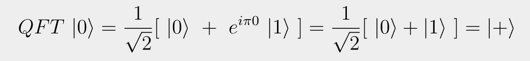
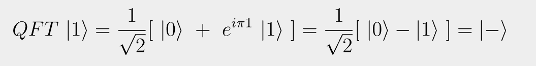
The Hadamard gate H is a 2×2 unitary matrix that maps each computational basis state to an equal superposition:

H  =  (1/√2)    +1   +1 
 +1   −1 

Applying H to each basis state:

InputH |input⟩Short name
|0⟩(1/√2)( |0⟩ + |1⟩ )|+⟩
|1⟩(1/√2)( |0⟩ |1⟩ )|−⟩

Both outputs have equal amplitudes of 1/√2, giving a 50% measurement probability for each outcome. The sign difference between |+⟩ and |−⟩ is what drives interference later.

Unitarity check: H†H = I. Since H is real and symmetric, H† = H, so H² = I. The Hadamard gate is its own inverse.

3  ·  H² = I: Quantum Interference

Applying H twice to |0⟩ returns the qubit to |0⟩. The algebra shows exactly why the |1⟩ amplitudes cancel through destructive interference:

H(H|0⟩)
  = H( (1/√2)(|0⟩ + |1⟩) )
  = (1/√2)( H|0⟩ + H|1⟩ )
  = (1/√2)( (1/√2)(|0⟩+|1⟩) + (1/√2)(|0⟩−|1⟩) )
  = (1/2)( |0⟩ + |1⟩ + |0⟩ − |1⟩ )
  = (1/2)( 2|0⟩ )
  = |0⟩ ✓
The +|1⟩ and −|1⟩ terms cancel completely (destructive interference) while the |0⟩ terms add (constructive interference). This is the fundamental mechanism behind quantum algorithms: arranging amplitudes so wrong answers cancel and the correct answer survives.

4  ·  Single-Qubit Circuit: H–H–Measure

A single qubit routed through two Hadamard gates and then measured always returns 0 with 100% probability:

q_0: H H M
StepStateNotes
1. Initialise|ψ₀⟩ = |0⟩Ground state
2. First H|ψ₁⟩ = (1/√2)(|0⟩+|1⟩)Superposition: 50/50
3. Second H|ψ₂⟩ = |0⟩Interference collapses back
4. MeasureResult = 0100% probability
This is a concrete demonstration that superposition is not just probabilistic noise. The deterministic outcome of 0 is only possible because the two Hadamard gates interact through interference, a purely quantum effect with no classical analogue.

5  ·  Tensor Products and Multi-Qubit States

Multi-qubit systems are described using the tensor product (⊗). For two qubits, the four computational basis states are:

KetTensor formColumn vector
|00⟩|0⟩ ⊗ |0⟩[1, 0, 0, 0]ᵀ
|01⟩|0⟩ ⊗ |1⟩[0, 1, 0, 0]ᵀ
|10⟩|1⟩ ⊗ |0⟩[0, 0, 1, 0]ᵀ
|11⟩|1⟩ ⊗ |1⟩[0, 0, 0, 1]ᵀ

The tensor product of two vectors is computed by multiplying each element of the first vector by the entire second vector and stacking the results. For |0⟩ ⊗ |1⟩:

|0⟩ ⊗ |1⟩
  = [1, 0]ᵀ ⊗ [0, 1]ᵀ
  = [ 1×[0,1]ᵀ ]  =  [0, 1, 0, 0]ᵀ  = |01⟩
    [ 0×[0,1]ᵀ ]
Dimension growth: n qubits span a 2ⁿ-dimensional Hilbert space. A 3-qubit system already has 8 basis states; a 50-qubit system has 2⁵⁰ ≈ 10¹⁵, impossible to store classically.

6  ·  Two-Qubit Superposition: H⊗H on |00⟩

Applying independent Hadamard gates to both qubits starting from |00⟩:

q_0: H
q_1: H
(H⊗H)|00⟩
  = (H|0⟩) ⊗ (H|0⟩)
  = (1/√2)(|0⟩+|1⟩) ⊗ (1/√2)(|0⟩+|1⟩)
  = (1/2)( |00⟩ + |01⟩ + |10⟩ + |11⟩ )
All four two-qubit basis states appear with equal amplitude 1/2. Each has measurement probability (1/2)² = 25%. This is the two-qubit analogue of the uniform superposition that opens algorithms like Grover’s.

7  ·  Interference in a Two-Qubit H–H Circuit

Applying H⊗H twice to |00⟩ returns it to |00⟩. The interference analysis on each basis state shows the mechanism:

Input to 2nd H⊗HAfter (H⊗H)
|00⟩(1/2)( |00⟩ + |01⟩ + |10⟩ + |11⟩ )
|01⟩(1/2)( |00⟩ − |01⟩ + |10⟩ − |11⟩ )
|10⟩(1/2)( |00⟩ + |01⟩ − |10⟩ − |11⟩ )
|11⟩(1/2)( |00⟩ − |01⟩ − |10⟩ + |11⟩ )

The initial superposition has equal weight 1/2 on each of the four states. Summing contributions to each output:

Output stateAmplitude sum (× 1/4)Result
|00⟩+1 +1 +1 +14/4 = 1 ✓ constructive
|01⟩+1 −1 +1 −10 destructive
|10⟩+1 +1 −1 −10 destructive
|11⟩+1 −1 −1 +10 destructive
Only |00⟩ survives. This is the same interference structure that the Grover diffusion operator exploits at scale: constructive interference on the target state, destructive on all others.

8  ·  The H⊗H Matrix and Why It Matters

The combined H⊗H operator is a 4×4 Walsh-Hadamard matrix (scaled by 1/2). Its sign pattern is exactly the two-qubit case of the popcount rule derived in the Walsh-Hadamard post:

H⊗H  =  (1/2)    +1   +1   +1   +1 
 +1   −1   +1   −1 
 +1   +1   −1   −1 
 +1   −1   −1   +1 

Every quantum algorithm that achieves a speedup over classical computation does so through the same three-phase structure:

PhaseOperationPurpose
1. OpenHadamard on all qubitsCreate uniform superposition over all 2ⁿ states
2. OperateOracle / phase manipulationMark or bias the amplitude of the target answer
3. CloseHadamard again (+ measurement)Interference concentrates probability on the answer
The bottom line: the qubit and the Hadamard gate are the entry point to everything. Grover’s O(√N) search, Shor’s O((log N)³) factoring, and every other quantum speedup ultimately trace back to this interference mechanism operating at scale.
About the author

Malcolm Low is an Associate Professor at the Singapore Institute of Technology, writing on quantum computing, programming, and applied computing from Singapore.

Website: malcolmlow.com  ·  Singapore


Quantum Series 2026  ·  Built with Qiskit 1.x

✦ This article was generated with the assistance of Claude by Anthropic

Quantum Computing: CHSH Game Simulator and Bell’s Inequality

QUANTUM SERIES 2026
Exploring Quantum Entanglement: CHSH Game Simulator

Have you ever wondered how quantum mechanics defies everyday intuition? This project demonstrates one of the most striking phenomena in quantum physics: quantum entanglement and its ability to violate classical physics constraints through a playable cooperative game.

🎮 Try the CHSH Game Simulator  |  📂 View on GitHub


1 · What Is the CHSH Game in Quantum Computing?

The CHSH (Clauser-Horne-Shimony-Holt) game is a cooperative thought experiment that reveals the strange power of quantum entanglement. Two players, Alice and Bob, cannot communicate during the game but may share a pre-agreed strategy or, crucially, a pair of entangled qubits.

Player Receives from referee Outputs
Alice Random bit x Bit a
Bob Random bit y Bit b

They win if and only if:

(a + b) mod 2 = x × y
With classical strategies, Alice and Bob can win at most 75% of the time. With a quantum strategy using entangled qubits, they can reach approximately 85.4%, violating the classical bound.

2 · Bell’s Inequality and the CHSH Value

In 1964, John Bell proved that no local hidden variable theory can reproduce all predictions of quantum mechanics. The CHSH inequality formalises Bell’s theorem as a single testable number S:

Theory CHSH Value (S) Win Rate
Classical (any local strategy) S ≤ 2 75%
Quantum mechanics S = 2√2 ≈ 2.828 ~85.4%

This violation is not a loophole or a trick. It proves that the correlations produced by entangled qubits cannot be explained by any shared classical information, even with pre-agreed randomness. Loophole-free Bell test experiments confirm that quantum entanglement is a genuine physical phenomenon with no classical analogue.

3 · Measurement Angles and Quantum Correlation

The quantum advantage arises from choosing measurement bases at specific angles. For the standard |Φ+⟩ Bell state, the optimal angles are:

Player Input bit Measurement basis
Alice x = 0
Alice x = 1 45°
Bob y = 0 22.5°
Bob y = 1 −22.5°

The probability that Alice and Bob produce the same outcome is:

P(same) = cos²(δ)

where δ is the angle between their chosen measurement bases. This quantum correlation is what enables them to exceed the 75% classical ceiling. Different Bell states exhibit either parallel correlation (|Φ+⟩, |Ψ+⟩: qubits tend to give the same outcome) or orthogonal correlation (|Φ−⟩, |Ψ−⟩: one qubit effectively rotated 90° relative to the other). The simulator adjusts its probability calculations accordingly for each state.

🧪 4 · The Four Bell States

The simulator supports all four maximally entangled Bell states. Each uses optimised measurement angles to achieve the theoretical quantum win rate of ~85%.

State Definition Correlation
|Φ+⟩ (|00⟩ + |11⟩) / √2 Parallel
|Φ−⟩ (|00⟩ − |11⟩) / √2 Orthogonal
|Ψ+⟩ (|01⟩ + |10⟩) / √2 Parallel
|Ψ−⟩ (|01⟩ − |10⟩) / √2 Orthogonal

🎯 5 · CHSH Game Simulator Features

Feature Details
🎯 Interactive Visualization Real-time p5.js visualization showing the entangled state, Alice’s measurement collapse, and Bob’s final measurement. Coloured basis quadrants and correlation indicators included.
🎮 Strategy Comparison Switch between Classical (always outputs 0, max 75%) and Quantum (entangled qubits, ~85.4%) strategies in real time.
🎲 Flexible Input Controls Set Alice’s x and Bob’s y to Random or Fixed (0 or 1) to test specific measurement configurations.
📊 Real-Time Statistics Running totals for rounds played, wins, losses, and win percentage converging toward theoretical predictions.
🔄 Round History Navigation Step through previous rounds to review specific outcomes and trace the quantum measurement process.
Built with: React, p5.js, and Claude Code

6 · Try the Quantum Entanglement Simulator

A suggested sequence to build intuition:

  1. Open the simulator and select the Classical strategy. Run 100 rounds and watch the win rate converge toward 75%.
  2. Switch to the Quantum strategy with the |Φ+⟩ Bell state. Run another 100 rounds and observe the rate climb toward 85%.
  3. Try the other three Bell states. Note how each state’s correlation type (parallel vs orthogonal) affects the outcome distribution.
  4. Set Alice and Bob’s inputs to Fixed values to test individual measurement configurations and trace the correlation manually.
  5. Use Round History to step back through specific rounds and verify the win condition (a + b) mod 2 = x × y by hand.

7 · Open Source Code on GitHub

The complete source code is on GitHub. Contributions welcome: explore the code, report issues, suggest improvements, or fork it to build your own quantum visualisations.

Planned enhancements include a 3D Bloch sphere visualisation (Three.js), step-by-step animated transitions, an in-app educational tutorial, a mathematical deep-dive panel, and improved mobile layout.

The CHSH game demonstrates that quantum entanglement is not a mathematical abstraction but a measurable, observable phenomenon with no classical analogue. This simulator makes that phenomenon interactive and accessible to anyone curious about quantum mechanics.


QUANTUM SERIES 2026 · Quantum Entanglement and Bell Inequalities

✦ This article was generated with the assistance of Claude by Anthropic

About the author

Malcolm Low is an Associate Professor at the Singapore Institute of Technology, writing on quantum computing, programming, and applied computing from Singapore.

Website: malcolmlow.com  ·  Singapore

Quantum Fourier Transform (QFT) of a Single Qubit is Hadamard Transform

Below is the definition of QFT as illustrated in the YouTube lecture by Abraham Asfaw.

The LaTex code for the equation is as follows and also available here.

Latex
| \tilde{x} \rangle \equiv ~ QFT ~ |x \rangle ~ \equiv \frac{1}{\sqrt{N}}\sum_{y=0}^{N-1}{e^{\frac{2\pi ix y}{N}}} ~| y \rangle

For the one qubit case, N = 21 = 2:

Latex
| \tilde{x} \rangle \equiv ~ QFT ~ |x \rangle ~ \equiv \frac{1}{\sqrt{}N}\sum_{y=0}^{N-1}{e^{\frac{2\pi ix y}{N}}} ~| y \rangle

Latex
\frac{1}{\sqrt{2}}\sum_{y=0}^{1}{e^{\pi ix y}} ~| y \rangle = \frac{1}{\sqrt{2}}[~e^{i \pi x 0}~ | 0 \rangle ~ + ~ e^{i \pi x 1}~| 1 \rangle] = \frac{1}{\sqrt{2}}[~|0\rangle ~+~e^{i \pi x}~|1 \rangle~]

When x = 0:

Latex
QFT~| 0 \rangle = \frac{1}{\sqrt{2}}[~|0\rangle ~+~e^{i \pi 0}~|1 \rangle~] = \frac{1}{\sqrt{2}}[~| 0 \rangle + |1 \rangle~] = |+\rangle

When x = 1:


Latex
QFT~| 1 \rangle = \frac{1}{\sqrt{2}}[~|0\rangle ~+~e^{i \pi 1}~|1 \rangle~] = \frac{1}{\sqrt{2}}[~| 0 \rangle - |1 \rangle~] = |-\rangle

Hence the QFT of a single qubit is essentially the Hadamard transform.