Blog

Deutsch Algorithm Revisited: Quantum vs Classical Implementation in Qiskit

Part of the Quantum Computing: A Complete Learning Path series.

QUANTUM SERIES 2026
Quantum vs classical implementation of Deutsch’s Algorithm in Qiskit: same answer, half the queries.

The previous post covered the theory: four Boolean functions, the reversible oracle U_f, the phase-kickback derivation, and the single-query measurement result. This post puts it into running code. We implement the classical two-query approach and the quantum one-query approach side by side in Qiskit so the advantage is visible, not just promised.

1 · The Challenge

Given a black-box function f: {0,1} → {0,1}, determine whether it is constant (f(0) = f(1)) or balanced (f(0) ≠ f(1)).

Approach	Oracle queries required	Strategy
Classical	2	Evaluate f(0), then f(1), compare
Quantum (Deutsch)	1	Query in superposition, read phase via interference

The quantum advantage: instead of probing the function at individual inputs, the algorithm queries it at a superposition of both inputs simultaneously, then uses interference to extract a global property (constant vs balanced) with a single measurement.

2 · Oracle Functions

First we build the four oracle circuits. Each implements one of the four single-bit Boolean functions as a reversible quantum gate. The constant oracles ignore x; the balanced oracles use x as a control.

      from qiskit import QuantumCircuit, QuantumRegister, ClassicalRegister

      from qiskit_aer import AerSimulator

      def create_constant_oracle(constant_value):

          “””Creates a constant oracle (returns 0 or 1 for all inputs)”””

          oracle = QuantumCircuit(2, name=f”Constant_{constant_value}”)

          if constant_value == 1:

              oracle.x(1)  # Flip the output qubit

          return oracle

      def create_balanced_oracle(balance_type):

          “””Creates a balanced oracle”””

          oracle = QuantumCircuit(2, name=f”Balanced_{balance_type}”)

          if balance_type == ‘identity’:

              # f(x) = x

              oracle.cx(0, 1)

          elif balance_type == ‘negation’:

              # f(x) = NOT x

              oracle.x(0)

              oracle.cx(0, 1)

              oracle.x(0)

          return oracle

3 · Classical Approach: Two Queries Required

The classical algorithm calls the oracle twice: once with input 0 to learn f(0), and once with input 1 to learn f(1). Each query is a separate circuit run.

      def classical_deutsch_query1(oracle):

          “””First query: Evaluate f(0)”””

          qr = QuantumRegister(2, ‘q’)

          cr = ClassicalRegister(1, ‘c’)

          qc = QuantumCircuit(qr, cr)

          # Input: x = 0 (already initialised to |0>)

          qc.barrier()

          qc.compose(oracle, inplace=True)

          qc.barrier()

          qc.measure(1, 0)  # Measure output to get f(0)

          return qc

      def classical_deutsch_query2(oracle):

          “””Second query: Evaluate f(1)”””

          qr = QuantumRegister(2, ‘q’)

          cr = ClassicalRegister(1, ‘c’)

          qc = QuantumCircuit(qr, cr)

          qc.x(0)  # Input: x = 1

          qc.barrier()

          qc.compose(oracle, inplace=True)

          qc.barrier()

          qc.measure(1, 0)  # Measure output to get f(1)

          return qc

Classical bottleneck: two separate measurements, two separate circuit executions. The classical algorithm measures the output qubit q[1] in both cases to read the function values directly.

4 · Quantum Approach: One Query Suffices

The quantum circuit initialises q[1] = |1⟩, applies Hadamard gates to both wires, queries the oracle exactly once, then applies a final Hadamard to q[0] before measuring it. The oracle is never called again.

      def deutsch_algorithm(oracle):

          “””Implements Deutsch’s algorithm — requires only ONE query”””

          qr = QuantumRegister(2, ‘q’)

          cr = ClassicalRegister(1, ‘c’)

          qc = QuantumCircuit(qr, cr)

          # Step 1: Initialise q[1] to |1>

          qc.x(1)

          qc.barrier()

          # Step 2: Hadamard on both wires (superposition)

          qc.h(0)

          qc.h(1)

          qc.barrier()

          # Step 3: Single oracle query

          qc.compose(oracle, inplace=True)

          qc.barrier()

          # Step 4: Final Hadamard on q[0]

          qc.h(0)

          qc.barrier()

          # Step 5: Measure q[0] — the INPUT qubit, not the output

          qc.measure(0, 0)

          return qc

The quantum circuit measures q[0], the input qubit. The classical circuits measure q[1], the output qubit. That structural difference is the entire quantum advantage: the quantum algorithm reads a global property of the function via interference, not an individual function value.

5 · Running the Comparison

Test all four oracles with both approaches and compare query counts.

      oracles = [

          (“Constant 0”,           create_constant_oracle(0)),

          (“Constant 1”,           create_constant_oracle(1)),

          (“Balanced (Identity)”, create_balanced_oracle(‘identity’)),

          (“Balanced (Negation)”, create_balanced_oracle(‘negation’))

      ]

      simulator = AerSimulator()

      for name, oracle in oracles:

          # Classical: 2 queries

          f_0 = int(list(simulator.run(classical_deutsch_query1(oracle), shots=1).result().get_counts().keys())[0])

          f_1 = int(list(simulator.run(classical_deutsch_query2(oracle), shots=1).result().get_counts().keys())[0])

          classical_result = “CONSTANT” if f_0 == f_1 else “BALANCED”

          # Quantum: 1 query

          counts = simulator.run(deutsch_algorithm(oracle), shots=1000).result().get_counts()

          quantum_result = “CONSTANT” if ‘0’ in counts else “BALANCED”

          print(f”{name}: Classical={classical_result}, Quantum={quantum_result}”)

Sample output:

      Constant 0:          Classical=CONSTANT, Quantum=CONSTANT

      Constant 1:          Classical=CONSTANT, Quantum=CONSTANT

      Balanced (Identity): Classical=BALANCED, Quantum=BALANCED

      Balanced (Negation): Classical=BALANCED, Quantum=BALANCED

Both methods always agree. The quantum result is deterministic: the simulator returns 100% |0⟩ for constant oracles and 100% |1⟩ for balanced ones, with zero noise on shots=1000.

6 · Circuit Overview

Classical Query 1 — Evaluate f(0)
q[0] stays in |0⟩, both wires pass through U_f, and q[1] is measured to read f(0).

          q[0]:
          
          |0⟩
          
          (not measured)
        
Uf

          q[1]:
          
          |0⟩
          
          M
          
          f(0)

Classical Query 2 — Evaluate f(1)
An X gate flips q[0] to |1⟩, both wires pass through U_f, and q[1] is measured to read f(1).

          q[0]:
          
          |0⟩
          
          X
          
          (not measured)
        
Uf

          q[1]:
          
          |0⟩
          
          M
          
          f(1)

Quantum Deutsch — Single Query
H gates create superposition on both wires, one oracle query encodes f(0) ⊕ f(1) as a phase, the final H on q[0] converts phase to amplitude, and measuring q[0] gives the answer directly.

          q[0]:
          
          |0⟩
          
          H
          
          H
          
          M
          
          0=const, 1=bal
        
Uf

          q[1]:
          
          |1⟩
          
          H

The structural difference: the classical circuits measure the output qubit q[1] to read individual function values. The quantum circuit measures the input qubit q[0] after interference to read a global property of the function. That is what lets a single query reveal whether the function is constant or balanced.

7 · Measurement Interpretation and Conclusion

The measurement result on q[0] maps directly to the function type:

Measure q[0]	Function type	Interference mechanism
0	Constant	f(0) ⊕ f(1) = 0 → constructive on \|0⟩
1	Balanced	f(0) ⊕ f(1) = 1 → destructive on \|0⟩, constructive on \|1⟩

The quantum speedup is 2x here (one query instead of two). Modest for a two-input function, but the same technique scales: Deutsch-Jozsa extends this to n-bit functions, cutting 2ⁿ⁻¹+1 classical queries down to one. Simon’s algorithm extends it further. Shor’s algorithm for factoring, the most consequential quantum algorithm known, relies on the same architectural idea: query in superposition, encode information as phase, extract via interference and measurement.

To run the code: pip install qiskit qiskit-aer. The full comparison script outputs all four oracle types side by side. Try modifying the oracle functions to explore how each gate sequence implements f.

Quantum Series 2026 · Built with Qiskit 1.x

✦ This article was generated with the assistance of Claude by Anthropic ✦

Continue the Quantum Series
← Deutsch’s four cases
View the complete Quantum Computing learning path
→ Reversible computation

December 20, 2025

Deutsch’s Algorithm in Quantum Computing: The 4 Cases

Part of the Quantum Computing: A Complete Learning Path series.

QUANTUM SERIES 2026
The four Boolean functions, the reversible oracle, and the single-query Deutsch circuit with full derivation.

Deutsch’s Algorithm determines whether a single-bit function f(x) is constant (f(0) = f(1)) or balanced (f(0) ≠ f(1)) using only one oracle query. To understand how the algorithm works, we first need to see how each possible function is physically realised as a reversible quantum gate, and then how the complete Deutsch circuit encodes that function into a measurable phase difference.

1 · The 4 Possible Functions

With a single input bit x ∈ {0,1} and output bit f(x) ∈ {0,1}, there are exactly four possible Boolean functions. Two are constant (output ignores the input) and two are balanced (output depends on the input).

#	Name	f(0)	f(1)	Gate implementation	Type
1	Constant Zero	0	0	Identity — no gates needed	Constant
2	Constant One	1	1	X gate on output wire only	Constant
3	Balanced ID	0	1	CNOT (x = control, y = target)	Balanced
4	Balanced NOT	1	0	X on x, CNOT, X on x (flip, copy, restore)	Balanced

The two balanced oracles as quantum circuits. Both have x on the control wire and y on the target wire, with the bottom wire carrying y ⊕ f(x) as output.

Balanced ID — f(x) = x

          x:
          
          control — x unchanged
        
          y:
          
          +
          
          y ⊕ x = y ⊕ f(x)

Balanced NOT — f(x) = ¬x

          x:
          
          X
          
          X
          
          flip, control, restore
        
          y:
          
          +
          
          y ⊕ ¬x = y ⊕ f(x)

Key point: both constant oracles leave the x wire untouched and act only on y. Both balanced oracles use x as a control and output y ⊕ f(x) on the target wire. All four are reversible, which is required for quantum computation.

2 · The General Oracle U_f

All four functions are wrapped in a single reversible gate U_f that leaves the input register unchanged and XORs the function value into the output register:

      Uf |x⟩|y⟩  =  |x⟩ |y ⊕ f(x)⟩
    

As a two-wire circuit, U_f passes x unchanged on the top wire while the bottom wire carries y ⊕ f(x). The box spans both wires to show they are processed jointly by a single gate:

          x:
          
          x (unchanged)
        
Uf

          y:
          
          y ⊕ f(x)

The reversibility of U_f is guaranteed because XOR is its own inverse: applying U_f twice returns the original state. This property allows quantum algorithms to query f without destroying the superposition.

Setting y = |−⟩ = (1/√2)(|0⟩ − |1⟩) turns U_f into a phase-kickback machine: U_f|x⟩|−⟩ = (−1)^f(x)|x⟩|−⟩. The function value is encoded in the phase of the control qubit rather than the target, and the target remains in |−⟩ unchanged.

3 · The Complete Deutsch Circuit

The algorithm wraps U_f in Hadamard gates on both wires. Initialise q[0] = |0⟩ and q[1] = |1⟩, apply H to both, query U_f once, apply a final H to q[0], then measure q[0]:

The three states at each checkpoint:

State	Expression	Note
\|ψ₀⟩	\|0⟩\|1⟩	Initialisation
\|ψ₁⟩	\|+⟩\|−⟩ = ½(\|0⟩+\|1⟩)(\|0⟩−\|1⟩)	After both H gates
\|ψ₂⟩	(1/√2)[(−1)^f(0)\|0⟩+(−1)^f(1)\|1⟩] ⊗ \|−⟩	After U_f, before final H

The target qubit q[1] stays in |−⟩ throughout. Only the phase of q[0] changes, carrying the function information via kickback.

4 · Mathematical Proof

The full derivation follows four steps. Each is exact; no approximation is involved.

      Step 1 — Initialisation:

        |ψ₀⟩ = |0⟩|1⟩

      Step 2 — Apply H to both wires:

        |ψ₁⟩ = |+⟩|−⟩

             = (1/√2)(|0⟩ + |1⟩) ⊗ (1/√2)(|0⟩ − |1⟩)

      Step 3 — Apply U_f (phase kickback on |−⟩ target):

        U_f |x⟩|−⟩ = (−1)^f(x) |x⟩|−⟩

        |ψ₂⟩ = (1/√2)[ (−1)^f(0)|0⟩ + (−1)^f(1)|1⟩ ] ⊗ |−⟩

      Step 4 — Apply H to q[0] and inspect cases:

        Constant  f(0) = f(1) = c:

          |ψ₂⟩ = (−1)^c (1/√2)(|0⟩ + |1⟩) ⊗ |−⟩

          After H: (−1)^c |0⟩ ⊗ |−⟩  →  Measure 0

        Balanced  f(0) ≠ f(1):

          |ψ₂⟩ = ±(1/√2)(|0⟩ − |1⟩) ⊗ |−⟩

          After H: ±|1⟩ ⊗ |−⟩  →  Measure 1

The global phase (−1)^c in the constant case is unobservable. All that matters is whether the amplitudes on |0⟩ and |1⟩ are in phase (constant) or out of phase (balanced), which the final H converts to a deterministic measurement.

5 · Final Measurement

The measurement of q[0] after the final Hadamard gives a deterministic result in both cases:

Measure q[0]	Function type	Why
0	Constant	f(0) ⊕ f(1) = 0; amplitudes add constructively on \|0⟩
1	Balanced	f(0) ⊕ f(1) = 1; amplitudes cancel on \|0⟩, survive on \|1⟩

A classical algorithm must evaluate f(0) and f(1) separately, requiring two queries. Deutsch’s algorithm queries U_f exactly once, using superposition to probe both inputs simultaneously and interference to extract a global property of the function. This is the first demonstrated quantum computational advantage over any classical approach.

The technique introduced here — query in superposition, encode information as phase, extract via interference — is the blueprint for Deutsch-Jozsa, Simon’s algorithm, and ultimately Shor’s factoring algorithm.

About the author

Malcolm Low is an Associate Professor at the Singapore Institute of Technology, writing on quantum computing, programming, and applied computing from Singapore.

Website: malcolmlow.com · Singapore

Quantum Series 2026 · Built with Qiskit 1.x

✦ This article was generated with the assistance of Claude by Anthropic ✦

Frequently Asked Questions

What is Deutsch’s algorithm?

Deutsch’s algorithm was the first quantum algorithm shown to outperform any classical algorithm. It determines whether a one-bit Boolean function is constant or balanced using a single query, versus the two queries a classical approach requires.

Why does Deutsch’s algorithm only need one query?

It uses phase kickback and superposition to evaluate the function on both possible inputs simultaneously, then uses interference to extract the answer from a single measurement.

What are the four cases in Deutsch’s algorithm?

The four possible one-bit Boolean functions are: always return 0, always return 1, return the input unchanged, and return the input’s negation. The first two are “constant,” the last two are “balanced.”

Is Deutsch’s algorithm useful in practice?

Not directly — it solves a toy problem — but it demonstrates the core quantum principles (superposition, interference, phase kickback) that underlie every practical quantum algorithm, including Grover’s and Shor’s.

Continue the Quantum Series
← Phase kickback
View the complete Quantum Computing learning path
→ Deutsch algorithm in Qiskit

December 9, 2025

Understanding Phase Kickback in Quantum Computing

Part of the Quantum Computing: A Complete Learning Path series.

QUANTUM SERIES 2026
How the target controls the controller and why this underpins Grover’s, Shor’s, and Deutsch’s algorithms.

In standard classical logic, a control bit dictates what happens to a target. In quantum mechanics the relationship is symmetric. When the target qubit is in an eigenstate of the gate operator, the eigenvalue phase is kicked back onto the control qubit, leaving the target unchanged while flipping the relative phase of the control. This post derives that result from first principles using the CNOT gate on |+⟩ ⊗ |−⟩.

1 · The CNOT Circuit and the Kickback Setup

The circuit places the control qubit in superposition |+⟩ and the target qubit in |−⟩. Since |−⟩ is an eigenstate of X with eigenvalue −1, the kickback occurs.

    control:
    
    |+⟩
    
    |−⟩
  
    target:
    
    |−⟩
    
    +
    
    |−⟩

Key observation: The target qubit is unchanged after the CNOT. The control qubit flips from |+⟩ to |−⟩. The phase was kicked back to the control, not forward to the target.

2 · Full Derivation: |+⟩ ⊗ |−⟩ through CNOT

Step 1 — Define the initial state

|ψ₀⟩ = |+⟩ ⊗ |−⟩
  = (1/√2)(|0⟩ + |1⟩) ⊗ (1/√2)(|0⟩ − |1⟩)

Step 2 — Expand the tensor product

|ψ₀⟩ = (1/2)[ |00⟩ − |01⟩ + |10⟩ − |11⟩ ]

Step 3 — Apply the CNOT gate

|ψ₁⟩ = (1/2)[ |00⟩ − |01⟩ + |11⟩ − |10⟩ ]

Step 4 — Factor and identify the result

|ψ₁⟩ = (1/2)[ |0⟩(|0⟩ − |1⟩) − |1⟩(|0⟩ − |1⟩) ]
  = (1/√2)(|0⟩ − |1⟩) ⊗ (1/√2)(|0⟩ − |1⟩)
  = |−⟩ ⊗ |−⟩

The target qubit is still |−⟩ — unchanged by the CNOT. The control qubit changed from |+⟩ to |−⟩. The −1 eigenvalue of the target has been kicked back as a relative phase onto the control.

3 · Why Phase Kickback Matters

The math shows that while we applied a gate to the target, the relative phase of the control qubit changed from positive to negative. This is a structural property of controlled unitaries acting on their eigenstates, and it appears at the core of every major quantum algorithm.

Algorithm	How phase kickback is used
Deutsch’s Algorithm	The oracle kicks a −1 phase onto the control qubit to encode whether f is constant or balanced, extractable with a single H gate measurement.
Grover’s Algorithm	The oracle flips the sign of the target state’s amplitude by kicking a −1 phase back to the control register, enabling amplitude amplification.
Shor’s Algorithm	Quantum Phase Estimation relies entirely on phase kickback to transfer eigenvalue information from the target register to the control register.

The general rule: for any unitary U with eigenstate |u⟩ (so U|u⟩ = eⁱᵖ|u⟩), a controlled-U gate with the control in superposition kicks the phase eⁱᵖ back to the control qubit. The target is unchanged.

About the author

Malcolm Low is an Associate Professor at the Singapore Institute of Technology, writing on quantum computing, programming, and applied computing from Singapore.

Website: malcolmlow.com · Singapore

Quantum Series 2026 · Built with Qiskit 1.x

✦ This article was generated with the assistance of Claude by Anthropic ✦

Frequently Asked Questions

What is phase kickback in quantum computing?

Phase kickback is a mechanism where applying a controlled operation causes a phase to appear on the control qubit rather than the target qubit, effectively transferring information “backward” through the circuit.

Why is phase kickback important?

It’s the underlying trick behind many quantum algorithms — including Deutsch’s, Grover’s, and Shor’s — because it lets a circuit encode information about a function’s global behavior into a measurable phase rather than needing to inspect every output individually.

How does phase kickback relate to Deutsch’s algorithm?

Deutsch’s algorithm uses phase kickback to write the result of evaluating a function onto the control qubit’s phase, allowing the answer to be extracted with a single query instead of the two a classical approach would need.

Continue the Quantum Series
← Qubits and Hadamard gates
View the complete Quantum Computing learning path
→ Deutsch’s algorithm

December 9, 2025

Does Challenging AI Make It Smarter?

A recent Medium article claims that adding challenge phrases like “I bet you can’t solve this” to AI prompts improves output quality by 45%, based on research by Li et al. (2023).

Quick Test Results

Testing these techniques on academic tasks—SQL queries, code debugging, and research synthesis—showed mixed but interesting results:

What worked: Challenge framing produced more thorough, systematic responses for complex multi-step problems. Confidence scoring (asking AI to rate certainty and re-evaluate if below 0.9) caught overconfident answers.

What didn’t: Simple factual queries showed no improvement.

The Why

High-stakes language doesn’t trigger AI emotions—it cues pattern-matching against higher-quality training examples where stakes were high.

Bottom Line

Worth trying for complex tasks, but expect higher token usage. Results are task-dependent, not universal.

Source: Li et al. (2023), arXiv:2307.11760

“`

Source: Li et al. (2023), arXiv:2307.11760

November 29, 2025

Introduction to Quantum Computing: Qubits, Hadamard Gates, and Superposition

Part of the Quantum Computing: A Complete Learning Path series.

QUANTUM SERIES 2026
Qubits, the Hadamard gate, superposition, tensor products, and quantum interference from first principles.

Classical computers store information in bits that are always exactly 0 or 1. Quantum computers exploit the principles of quantum mechanics to do something fundamentally different: they operate on qubits, which can exist in a superposition of both states simultaneously. The Hadamard gate is the simplest gate that creates this superposition, and understanding it from first principles is the entry point to every quantum algorithm that follows.

1 · The Qubit

A qubit is the fundamental unit of quantum information. Unlike a classical bit, a qubit can exist in a superposition of |0⟩ and |1⟩ simultaneously. We write its general state using Dirac (bra-ket) notation:

|ψ⟩ = α|0⟩ + β|1⟩

Here α and β are complex numbers called probability amplitudes. They must satisfy the normalisation condition:

|α|² + |β|² = 1

The two computational basis states are represented as column vectors:

When we measure the qubit in state |ψ⟩ = α|0⟩ + β|1⟩, we get |0⟩ with probability |α|² and |1⟩ with probability |β|². The act of measurement destroys the superposition and collapses the qubit to a definite classical state.

Key distinction: The superposition is not just ignorance about a hidden value. The qubit genuinely occupies both states until measured, and this physical reality is what quantum algorithms exploit.

2 · The Hadamard Gate

The Hadamard gate H is a 2×2 unitary matrix that maps each computational basis state to an equal superposition:

      H  =  (1/√2)  
       +1   +1 
 +1   −1 
    

Applying H to each basis state:

Input	H \|input⟩	Short name
\|0⟩	(1/√2)( \|0⟩ + \|1⟩ )	\|+⟩
\|1⟩	(1/√2)( \|0⟩ − \|1⟩ )	\|−⟩

Both outputs have equal amplitudes of 1/√2, giving a 50% measurement probability for each outcome. The sign difference between |+⟩ and |−⟩ is what drives interference later.

Unitarity check: H†H = I. Since H is real and symmetric, H† = H, so H² = I. The Hadamard gate is its own inverse.

3 · H² = I: Quantum Interference

Applying H twice to |0⟩ returns the qubit to |0⟩. The algebra shows exactly why the |1⟩ amplitudes cancel through destructive interference:

      H(H|0⟩)

        = H( (1/√2)(|0⟩ + |1⟩) )

        = (1/√2)( H|0⟩ + H|1⟩ )

        = (1/√2)( (1/√2)(|0⟩+|1⟩) + (1/√2)(|0⟩−|1⟩) )

        = (1/2)( |0⟩ + |1⟩ + |0⟩ − |1⟩ )

        = (1/2)( 2|0⟩ )

        = |0⟩ ✓

The +|1⟩ and −|1⟩ terms cancel completely (destructive interference) while the |0⟩ terms add (constructive interference). This is the fundamental mechanism behind quantum algorithms: arranging amplitudes so wrong answers cancel and the correct answer survives.

4 · Single-Qubit Circuit: H–H–Measure

A single qubit routed through two Hadamard gates and then measured always returns 0 with 100% probability:

Step	State	Notes
1. Initialise	\|ψ₀⟩ = \|0⟩	Ground state
2. First H	\|ψ₁⟩ = (1/√2)(\|0⟩+\|1⟩)	Superposition: 50/50
3. Second H	\|ψ₂⟩ = \|0⟩	Interference collapses back
4. Measure	Result = 0	100% probability

This is a concrete demonstration that superposition is not just probabilistic noise. The deterministic outcome of 0 is only possible because the two Hadamard gates interact through interference, a purely quantum effect with no classical analogue.

5 · Tensor Products and Multi-Qubit States

Multi-qubit systems are described using the tensor product (⊗). For two qubits, the four computational basis states are:

Ket	Tensor form	Column vector
\|00⟩	\|0⟩ ⊗ \|0⟩	[1, 0, 0, 0]ᵀ
\|01⟩	\|0⟩ ⊗ \|1⟩	[0, 1, 0, 0]ᵀ
\|10⟩	\|1⟩ ⊗ \|0⟩	[0, 0, 1, 0]ᵀ
\|11⟩	\|1⟩ ⊗ \|1⟩	[0, 0, 0, 1]ᵀ

The tensor product of two vectors is computed by multiplying each element of the first vector by the entire second vector and stacking the results. For |0⟩ ⊗ |1⟩:

      |0⟩ ⊗ |1⟩

        = [1, 0]ᵀ ⊗ [0, 1]ᵀ

        = [ 1×[0,1]ᵀ ]  =  [0, 1, 0, 0]ᵀ  = |01⟩

          [ 0×[0,1]ᵀ ]

Dimension growth: n qubits span a 2ⁿ-dimensional Hilbert space. A 3-qubit system already has 8 basis states; a 50-qubit system has 2⁵⁰ ≈ 10¹⁵, impossible to store classically.

6 · Two-Qubit Superposition: H⊗H on |00⟩

Applying independent Hadamard gates to both qubits starting from |00⟩:

        q_0:
        
        H

        q_1:
        
        H

      (H⊗H)|00⟩

        = (H|0⟩) ⊗ (H|0⟩)

        = (1/√2)(|0⟩+|1⟩) ⊗ (1/√2)(|0⟩+|1⟩)

        = (1/2)( |00⟩ + |01⟩ + |10⟩ + |11⟩ )

All four two-qubit basis states appear with equal amplitude 1/2. Each has measurement probability (1/2)² = 25%. This is the two-qubit analogue of the uniform superposition that opens algorithms like Grover’s.

7 · Interference in a Two-Qubit H–H Circuit

Applying H⊗H twice to |00⟩ returns it to |00⟩. The interference analysis on each basis state shows the mechanism:

Input to 2nd H⊗H	After (H⊗H)
\|00⟩	(1/2)( \|00⟩ + \|01⟩ + \|10⟩ + \|11⟩ )
\|01⟩	(1/2)( \|00⟩ − \|01⟩ + \|10⟩ − \|11⟩ )
\|10⟩	(1/2)( \|00⟩ + \|01⟩ − \|10⟩ − \|11⟩ )
\|11⟩	(1/2)( \|00⟩ − \|01⟩ − \|10⟩ + \|11⟩ )

The initial superposition has equal weight 1/2 on each of the four states. Summing contributions to each output:

Output state	Amplitude sum (× 1/4)	Result
\|00⟩	+1 +1 +1 +1	4/4 = 1 ✓ constructive
\|01⟩	+1 −1 +1 −1	0 destructive
\|10⟩	+1 +1 −1 −1	0 destructive
\|11⟩	+1 −1 −1 +1	0 destructive

Only |00⟩ survives. This is the same interference structure that the Grover diffusion operator exploits at scale: constructive interference on the target state, destructive on all others.

8 · The H⊗H Matrix and Why It Matters

The combined H⊗H operator is a 4×4 Walsh-Hadamard matrix (scaled by 1/2). Its sign pattern is exactly the two-qubit case of the popcount rule derived in the Walsh-Hadamard post:

      H⊗H  =  (1/2)  
      
         +1   +1   +1   +1 

         +1   −1   +1   −1 

         +1   +1   −1   −1 

         +1   −1   −1   +1

Every quantum algorithm that achieves a speedup over classical computation does so through the same three-phase structure:

Phase	Operation	Purpose
1. Open	Hadamard on all qubits	Create uniform superposition over all 2ⁿ states
2. Operate	Oracle / phase manipulation	Mark or bias the amplitude of the target answer
3. Close	Hadamard again (+ measurement)	Interference concentrates probability on the answer

The bottom line: the qubit and the Hadamard gate are the entry point to everything. Grover’s O(√N) search, Shor’s O((log N)³) factoring, and every other quantum speedup ultimately trace back to this interference mechanism operating at scale.

About the author

Malcolm Low is an Associate Professor at the Singapore Institute of Technology, writing on quantum computing, programming, and applied computing from Singapore.

Website: malcolmlow.com · Singapore

Quantum Series 2026 · Built with Qiskit 1.x

✦ This article was generated with the assistance of Claude by Anthropic ✦

Hadamard tensor products and multiple qubits: quick answers

What is a Hadamard tensor product?

The Hadamard tensor product combines independent Hadamard gates into one operation for multiple qubits. For two qubits, H ⊗ H is a 4 × 4 matrix. Applied to |00⟩, it creates an equal superposition: (|00⟩ + |01⟩ + |10⟩ + |11⟩)/2. Each basis state therefore has amplitude 1/2 and measurement probability 1/4.

How does the Hadamard gate work on multiple qubits?

Applying H to each of n qubits is written H^⊗n. Starting with |0⟩^⊗n, it produces an equal superposition of all 2ⁿ computational basis states, each with amplitude 1/√(2ⁿ). This prepares the search space used by algorithms such as Deutsch’s and Grover’s algorithms.

Does a Hadamard tensor product create entanglement?

Not by itself. Independent Hadamard gates create a separable superposition. Entanglement requires an interaction between qubits, such as a controlled-NOT gate.

Continue the Quantum Series

Next, see Deutsch’s algorithm and its four cases, then study Grover’s inversion about the mean and the Walsh–Hadamard matrix in Grover’s diffusion operator. The complete sequence is collected in the Quantum Computing learning path.

Related interactive experiment: Ready to see entanglement outperform classical physics? Try the CHSH game simulator and compare the 75% classical limit with the 85.4% quantum strategy. Play and learn with the CHSH game.

Continue the Quantum Series
← CHSH entanglement simulator
View the complete Quantum Computing learning path
→ Phase kickback

November 27, 2025

Euler’s Formula: Why e^(iφ) Is Just Shorthand for a Circle

QUANTUM SERIES 2026
Foundational pre-reading: why e^iφ is just shorthand for a circle.

This is the foundational pre-reading for the upcoming Quantum Mechanics series. Before wave functions, probability amplitudes, and the quirks of qubits, one piece of mathematics has to be demystified: Euler’s formula. Quantum physics literature leans on the expression e^iφ, the phase factor, on almost every page. Raising a constant to an imaginary exponent looks intimidating at first, but conceptually it is nothing more than elegant shorthand for drawing a circle.

New to the math? Read top to bottom. Comfortable with the complex plane already? Skip ahead to Section 4 to see why quantum mechanics relies on this shorthand.

1 · The geometry: mapping the complex plane

On a standard 2D graph, points are plotted against an x-axis and a y-axis. The complex plane keeps the layout but changes the meaning: the horizontal axis measures real numbers, and the vertical axis measures imaginary numbers, the multiples of i. Draw a unit circle, a circle of radius 1, and any point on it is fixed by a single angle φ measured counter-clockwise from the positive real axis. Basic trigonometry gives its two coordinates: the horizontal coordinate is cos φ and the vertical coordinate is sin φ. Placed in the complex plane, that point is the real part plus i times the imaginary part, which is exactly Euler’s formula:

e^iφ = cos φ + i sin φ

Re

Im

e^iφ

φ

cos φ

sin φ

1

Fig 1: a point e^iφ on the unit circle. Its horizontal coordinate is cos φ, its vertical coordinate is sin φ.

As φ increases from 0 to 2π, the point sweeps out a full circle around the origin. The right-hand side spells out the coordinates; the left-hand side, the exponential, is the shorthand for the same thing.

2 · The mechanics of i: the ultimate rotator

Why should a circle be written as an exponent? The answer starts by reframing the imaginary unit. Algebraically i is the square root of minus one. Geometrically, multiplying any number by i rotates it 90 degrees counter-clockwise in the complex plane. Start at 1, pointing right. One multiplication by i gives i, pointing straight up. Another gives −1, pointing left. Two more pass through −i and return to 1.

1 ×i → i ×i → −1 ×i → −i ×i → 1
each ×i is a 90° counter-clockwise turn

Seen this way, i is not really a number at all. It is a rotational operator.

3 · The calculus: why the base e?

The base e earns its place through calculus: e^x is the only function that is its own derivative, so its rate of change always equals its current value. Feeding the rotational operator i into the exponent and differentiating by the chain rule gives:

ddφ e^iφ = i e^iφ

That small equation carries a large physical statement. The velocity of the point, the direction it is moving, equals its current position multiplied by i, which means the velocity is always exactly 90 degrees away from the position vector.

90°

e^iφ

i·e^iφ

Fig 2: the velocity i·e^iφ is the position vector turned 90°, so it stays tangent to the circle. Perpetual perpendicular velocity is exactly circular motion.

In geometry and orbital mechanics alike, a velocity that stays perpendicular to the position vector is the signature of perfect circular motion. The exponential therefore encodes the act of tracing a circle, automatically.

4 · Why quantum mechanics needs this

Rather than writing out a vector built from a real cosine component and an imaginary sine component every time, physicists write the phase factor and move on. The shorthand packs the coordinates, the radius, and the continuous rotation into one compact exponent. The next articles in this series turn to quantum superposition, where relative phase decides whether amplitudes interfere constructively or destructively. Because that relative phase behaves exactly like an angle travelling around a circle, e^iφ is the natural tool for modelling it.

Quantum Series 2026 · Foundational pre-reading

✦ Drafted with Gemini by Google, formatted and illustrated with Claude by Anthropic ✦

November 26, 2025

Mac Studio vs Mac Mini M4: Local AI Performance Benchmarks

APPLE SILICON 2025
Mac Studio vs Mac Mini M4: Local AI Performance Benchmarks

The rise of local AI has transformed how professionals and enthusiasts interact with large language models. Running AI models locally offers significant advantages: complete data privacy, no recurring subscription costs, offline functionality, and freedom from rate limits. However, the performance of local AI systems varies dramatically depending on hardware choices.

Apple Silicon has emerged as a compelling platform for local AI deployment, leveraging unified memory architecture and efficient neural processing capabilities. But which Apple system delivers the best balance of performance, capability, and value for running local language models?

1 · Motivation

Choosing the right hardware for local AI can be challenging. While cloud-based AI services like ChatGPT and Claude offer convenience, they come with privacy concerns, ongoing costs, and dependency on internet connectivity. Local AI eliminates these issues but requires careful hardware selection to ensure adequate performance.

This benchmark comparison aims to answer four critical questions:

How does the Mac Studio compare to the more affordable Mac Mini M4?
What performance trade-offs exist when scaling from tiny (1B) to medium (14B) models?
Which configurations provide acceptable interactive performance?
Where do Apple Silicon systems stand compared to dedicated GPU solutions?

All benchmarks were conducted using LocalScore AI, a standardized testing platform measuring generation speed, response latency, and prompt processing capabilities. Tests were run on November 13, 2025 using Q4_K Medium quantization.

2 · Key Takeaway

The Mac Studio dominates local AI performance across all model sizes, delivering 2–10x better speeds than the Mac Mini M4 depending on configuration.

Quick Recommendation: Choose Mac Studio for professional work or if you want to run 8B+ models. Choose Mac Mini M4 only if you are budget-constrained and committed to tiny (1B) models exclusively.

3 · Complete Performance Results

Both systems were tested with tiny (1B), small (8B), and medium (14B) models using Q4_K Medium quantization.

Metric	Mac Studio (1B)	Mac Mini M4 (1B)	Mac Studio (8B)	Mac Mini M4 (8B)	Mac Studio (14B)	Mac Mini M4 (14B)
Model	Llama 3.2 1B	Llama 3.2 1B	Llama 3.1 8B	Llama 3.1 8B	Qwen2.5 14B	Qwen2.5 14B
Generation Speed	178 tokens/s	77.1 tokens/s	62.7 tokens/s	17.7 tokens/s	35.8 tokens/s	9.6 tokens/s
Time to First Token	203 ms	1,180 ms	1,060 ms	6,850 ms	2,040 ms	13,300 ms
Prompt Processing	5,719 tokens/s	1,111 tokens/s	1,119 tokens/s	186 tokens/s	583 tokens/s	96 tokens/s
LocalScore Rating	1,713	417	405	78	217	41

4 · Performance Analysis by Model Size

Tiny Model (1B Parameters)

Metric	Mac Studio	Mac Mini M4	Performance Ratio
Generation Speed	178 tokens/s	77.1 tokens/s	2.3x faster
Time to First Token	203 ms	1,180 ms	5.8x faster
Prompt Processing	5,719 tokens/s	1,111 tokens/s	5.1x faster
LocalScore Rating	1,713	417	4.1x higher

Mac Studio: Delivers exceptional performance with near-instantaneous 203 ms response time. Excellent for real-time coding assistance, content creation, and interactive workflows.

Mac Mini M4: Provides functional performance with noticeable 1.18-second latency. Adequate for occasional use and non-critical applications.

Small Model (8B Parameters)

Metric	Mac Studio	Mac Mini M4	Performance Ratio
Generation Speed	62.7 tokens/s	17.7 tokens/s	3.5x faster
Time to First Token	1,060 ms	6,850 ms	6.5x faster
Prompt Processing	1,119 tokens/s	186 tokens/s	6.0x faster
LocalScore Rating	405	78	5.2x higher

Mac Studio: Maintains functional performance with 1.06-second response time. Suitable for quality-focused applications where enhanced model capabilities justify slower speeds.

Mac Mini M4: Experiences severe degradation with 6.85-second latency, making interactive use impractical for most workflows.

Medium Model (14B Parameters)

Metric	Mac Studio	Mac Mini M4	Performance Ratio
Generation Speed	35.8 tokens/s	9.6 tokens/s	3.7x faster
Time to First Token	2,040 ms	13,300 ms	6.5x faster
Prompt Processing	583 tokens/s	96 tokens/s	6.1x faster
LocalScore Rating	217	41	5.3x higher

Mac Studio: Shows significant slowdown with 2.04-second response time. Best for batch-oriented workflows where maximum model capability is prioritised over speed.

Mac Mini M4: Performance becomes severely constrained with 13.3-second latency. Generation at only 9.6 tokens/s makes this configuration unusable for interactive applications.

5 · Model Scaling Performance

Mac Studio Scaling

Model Size	Generation	First Token	Prompt Processing	Score
1B (Tiny)	178 tokens/s	203 ms	5,719 tokens/s	1,713
8B (Small)	62.7 tokens/s	1,060 ms	1,119 tokens/s	405
14B (Medium)	35.8 tokens/s	2,040 ms	583 tokens/s	217

The Mac Studio shows progressive degradation as model size increases but maintains usable performance throughout. The 8x parameter increase from 1B to 8B results in 65% slower generation; the 14B model runs at approximately half the speed of the 8B.

Mac Mini M4 Scaling

Model Size	Generation	First Token	Prompt Processing	Score
1B (Tiny)	77.1 tokens/s	1,180 ms	1,111 tokens/s	417
8B (Small)	17.7 tokens/s	6,850 ms	186 tokens/s	78
14B (Medium)	9.6 tokens/s	13,300 ms	96 tokens/s	41

The Mac Mini M4 experiences catastrophic degradation with larger models. The jump from 1B to 8B results in 77% slower generation; the 14B adds a further 46% reduction. A 13.3-second time to first token makes the 14B configuration nearly unusable for any interactive application.

6 · Configuration Recommendations

Configuration	Performance	Best For	Rating
Mac Studio + 1B	178 tok/s, 203 ms	Real-time coding, content creation	Excellent
Mac Studio + 8B	62.7 tok/s, 1.06 s	Enhanced reasoning, quality work	Good
Mac Studio + 14B	35.8 tok/s, 2.04 s	Max capability, batch workflows	Fair
Mac Mini M4 + 1B	77.1 tok/s, 1.18 s	Budget-conscious, occasional use	Fair
Mac Mini M4 + 8B	17.7 tok/s, 6.85 s	Not suitable for interactive use	Poor
Mac Mini M4 + 14B	9.6 tok/s, 13.3 s	Not practical for any use case	Poor

7 · Bottom Line

The Mac Studio demonstrates clear superiority across all tested configurations, with performance advantages ranging from 2–6x for tiny models up to 10x for larger ones. The system handles tiny models exceptionally well, small models competently, and medium models adequately for users prioritising capability over speed.

The Mac Mini M4 is only viable for tiny (1B) models, where it provides functional if slower performance. Small (8B) and medium (14B) models push the hardware well beyond practical limits, with response latencies of 6.85 and 13.3 seconds making interactive use frustrating or impossible.

Hardware choice significantly impacts local AI usability. Match your investment to your model size requirements: Mac Studio for flexibility across all model sizes, Mac Mini M4 only if you are committed to tiny models exclusively.

8 · Apple Silicon vs Dedicated GPUs

While these benchmarks show the Mac Studio leading among Apple Silicon options, dedicated GPU solutions like the NVIDIA RTX 4090 still deliver 3–5x higher raw performance for similar model sizes, with 400+ tokens/s achievable on small models.

Apple Silicon remains compelling despite lower absolute throughput:

System Integration: All-in-one design without external GPU requirements
Energy Efficiency: Lower power consumption and heat generation
Silent Operation: Minimal fan noise compared to high-performance GPUs
Unified Memory: Efficient sharing between CPU and neural processing
macOS Ecosystem: Seamless integration with macOS applications and workflows

Users requiring maximum raw throughput should consider GPU-based systems. Those prioritising integration, efficiency, noise levels, and macOS compatibility will find Apple Silicon delivers excellent local AI capabilities within its design constraints.

For more hardware comparisons, visit LocalScore AI.

9 · Benchmark Sources

Hardware	Model	Parameters	Test Link
Mac Studio	Llama 3.2 1B	1B (Tiny)	Test #1788
Mac Mini M4	Llama 3.2 1B	1B (Tiny)	Test #1789
Mac Studio	Llama 3.1 8B	8B (Small)	Test #1790
Mac Mini M4	Llama 3.1 8B	8B (Small)	Test #1791
Mac Studio	Qwen2.5 14B	14B (Medium)	Test #1792
Mac Mini M4	Qwen2.5 14B	14B (Medium)	Test #1793

All tests conducted November 13, 2025, using LocalScore AI with Q4_K Medium quantization.

Apple Silicon 2025 · Local AI Benchmarks

✦ This article was generated with the assistance of Claude by Anthropic ✦

Frequently Asked Questions

Is Mac Studio better than Mac Mini M4 for local LLMs?

Yes — across every model size tested, Mac Studio delivered meaningfully faster generation and higher LocalScore ratings than Mac Mini M4, with the gap widening as model size increases.

How much faster is Mac Studio than Mac Mini M4 for AI workloads?

Generation speed ranged from roughly 2x faster on small 1B models to over 10x faster on larger models, with LocalScore ratings up to 5x higher on Mac Studio.

What size LLMs can run on a Mac Mini M4?

Mac Mini M4 can run smaller local models (roughly 1B–8B parameters) at usable speeds, but larger models see a steep drop-off in tokens/second compared to Mac Studio.

Is Mac Studio worth it for running local AI models?

If you regularly run 8B+ parameter models or want faster iteration, yes — the performance gap becomes substantial at larger model sizes, though Mac Mini remains a reasonable budget option for lighter workloads.

November 13, 2025

Homebrew Cask: What It Is and How to Install Mac Apps

Homebrew Cask is a command-line extension of Homebrew, the macOS package manager, that installs, updates, and removes full graphical (GUI) applications, things like Chrome, Slack, or VS Code, using a single terminal command instead of downloading a disk image and dragging an icon into Applications.

Homebrew Cask quick answer: use brew install --cask app-name to install a macOS GUI application from Terminal.

brew search --cask chrome
brew install --cask google-chrome
brew upgrade --cask
brew uninstall --cask google-chrome

macOS users frequently face the challenge of efficiently managing application installations across multiple machines. The traditional approach involves manually downloading disk images, navigating installation wizards, and maintaining applications across systems. Homebrew Cask offers a command-line solution that significantly streamlines this process.

What Is Homebrew Cask?

Homebrew installs command-line tools and libraries, called formulae, while Homebrew Cask installs complete macOS applications with graphical interfaces. For example, brew install wget installs a terminal utility, whereas brew install --cask visual-studio-code installs the Visual Studio Code app in macOS. Cask functionality is built into modern Homebrew, so no separate tap or extension needs to be installed.

The conventional installation workflow requires multiple steps:

Locating the official download source
Downloading the disk image file
Opening and mounting the disk image
Transferring the application to the Applications folder
Ejecting the disk image
Managing the downloaded installer file
Repeating this process for each required application

Homebrew Cask reduces this to a single command:

brew install --cask google-chrome

The application is then installed automatically with no further user interaction required.

Key Advantages for Professional Workflows

1. Accelerated System Provisioning

Organizations and individual users can maintain installation scripts containing all required applications. A typical enterprise development environment setup might include:

brew install --cask visual-studio-code
brew install --cask docker
brew install --cask slack
brew install --cask zoom
brew install --cask rectangle
brew install --cask iterm2
brew install --cask spotify
brew install --cask vlc

This approach reduces new machine setup time from several hours to approximately 15-20 minutes, depending on network bandwidth and the number of applications being installed.

2. Simplified Update Management

Maintaining current software versions is essential for security compliance and feature availability. Rather than monitoring and updating each application individually, administrators can execute a single command:

brew upgrade --cask

This command updates all Cask-managed applications to their latest versions, ensuring consistent patch management across the system.

3. Complete Application Removal

Standard macOS uninstallation methods often leave residual files including configuration data, cache files, and preference files distributed throughout the file system. Homebrew Cask performs thorough removal:

brew uninstall --cask docker

This ensures complete application removal without orphaned system files.

4. Automation and Standardization

Homebrew Cask’s command-line interface enables scripting and automation. Development teams can create standardized setup scripts ensuring consistent development environments. IT departments can implement automated workstation provisioning workflows. System configurations can be version-controlled in dotfiles repositories, enabling rapid deployment and rollback capabilities.

Recommended Applications by Category

The following applications represent commonly deployed tools across professional environments:

Development Tools

brew install --cask visual-studio-code
brew install --cask iterm2
brew install --cask docker
brew install --cask postman
brew install --cask dbeaver-community

Productivity Applications

brew install --cask rectangle        # Window management
brew install --cask alfred           # Enhanced search functionality
brew install --cask obsidian         # Knowledge management
brew install --cask notion           # Collaborative workspace

Communication Platforms

brew install --cask slack
brew install --cask zoom
brew install --cask discord

System Utilities

brew install --cask the-unarchiver
brew install --cask appcleaner
brew install --cask vlc

Implementation Guide

Organizations and users without an existing Homebrew installation can deploy it with a single command:

/bin/bash -c "$(curl -fsSL https://raw.githubusercontent.com/Homebrew/install/HEAD/install.sh)"

Once Homebrew is installed, Cask functionality is built right in. Just start using brew install --cask commands.

Useful Commands to Know

# Search for an app
brew search --cask chrome

# Get information about an app
brew info --cask visual-studio-code

# List all installed cask apps
brew list --cask

# Update all apps
brew upgrade --cask

# Uninstall an app
brew uninstall --cask slack

A Few Gotchas

Cask isn’t perfect. Here are some things to be aware of:

Not every app is available – Popular apps are well-covered, but niche or very new applications might not be in the repository yet
App Store apps aren’t included – Apps distributed exclusively through the Mac App Store can’t be installed via Cask
Some apps require manual steps – Occasionally, an app needs additional configuration or permissions that Cask can’t automate
Updates might lag slightly – Cask maintainers need to update formulas when new versions release, so there can be a brief delay

These are minor inconveniences compared to the time saved.

Frequently Asked Questions

What is a cask in Homebrew?

A “cask” is Homebrew’s term for a pre-packaged macOS GUI application, as opposed to a “formula,” which is Homebrew’s term for a command-line tool or library. When you run brew install --cask app-name, Homebrew downloads the official installer for that app and places it in Applications automatically, skipping the manual disk-image and drag-and-drop steps entirely.

What is the difference between Homebrew and Homebrew Cask?

Homebrew installs command-line tools and libraries (things like git or wget). Homebrew Cask is the same package manager extended to install full graphical applications (things like Chrome or Slack). Since 2018 they’ve shipped as a single unified brew command — you don’t need to install Cask separately, just add the --cask flag.

Is Homebrew Cask free?

Yes. Homebrew and Homebrew Cask are both free, open-source projects. There’s no cost to install or use them — you’re simply automating the download of each app’s own installer, which may itself be free or paid depending on the app.

How do I install an app with Homebrew Cask?

Run brew install --cask app-name in Terminal, replacing app-name with the app’s Cask identifier (for example, brew install --cask visual-studio-code). Use brew search --cask keyword first if you’re not sure of the exact name.

The Bottom Line

Homebrew Cask has fundamentally changed how I interact with my Mac. What started as a way to avoid repetitive downloads has become an essential part of my workflow. The ability to script, automate, and version-control my application setup means I’m never more than a few commands away from a productive environment.

If you spend any significant time on macOS, especially as a developer or power user, Homebrew Cask is worth learning. Your future self—the one setting up that next new machine—will thank you.

Try It Yourself

Pick three applications you use regularly and install them via Cask. I bet you’ll be hooked by the simplicity. Start with something like:

brew install --cask visual-studio-code
brew install --cask google-chrome  
brew install --cask rectangle

Welcome to a more efficient way of managing your Mac applications.

What’s your favorite Homebrew Cask application? Have you automated your Mac setup? Share your experiences in the comments below!

November 12, 2025

AI is displacing software engineers, but those in Singapore have the chance to fare better

https://www.straitstimes.com/business/ai-is-displacing-software-engineers-but-those-in-singapore-have-the-chance-to-fare-better?sfnsn=mo

October 20, 2025

CHSH Game Simulator: Bell’s Inequality and Quantum Entanglement

Part of the Quantum Computing: A Complete Learning Path series.

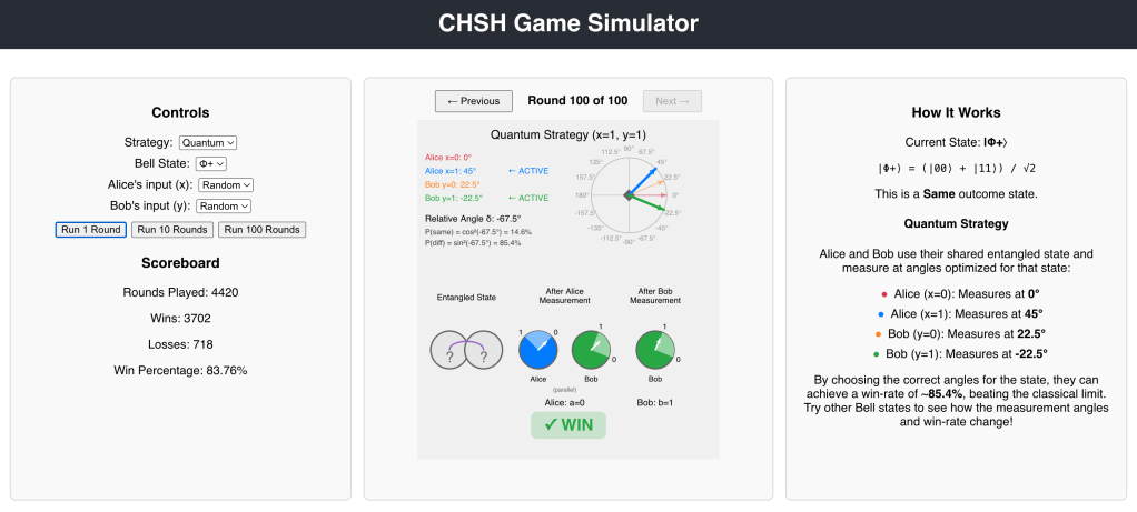
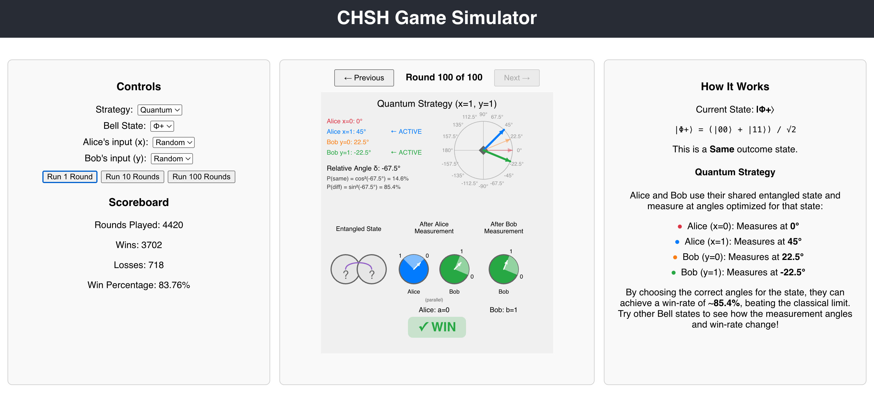
CHSH game simulator comparing classical and quantum entanglement strategies

QUANTUM SERIES 2026
Exploring Quantum Entanglement: CHSH Game Simulator

The CHSH game is a two-player experiment that demonstrates how quantum entanglement produces correlations impossible under classical physics. In this interactive CHSH game simulator, you can compare the classical maximum win rate of 75% with the quantum result of approximately 85.4%, explore all four Bell states, and see Bell’s inequality violated in real time.

🎮 Play the CHSH Game Simulator 📂 View Source on GitHub

1 · How to Play the CHSH Game

The CHSH (Clauser-Horne-Shimony-Holt) game is a cooperative thought experiment that reveals the strange power of quantum entanglement. Two players, Alice and Bob, cannot communicate during the game but may share a pre-agreed strategy or, crucially, a pair of entangled qubits.

The referee gives Alice a random input bit x and Bob a random input bit y.
Without communicating, Alice returns a and Bob returns b.
They win when a ⊕ b = x ∧ y: their answers match unless both input bits are 1.
Repeat many rounds and compare the classical and quantum win rates.

Player	Receives from referee	Outputs
Alice	Random bit x	Bit a
Bob	Random bit y	Bit b

They win if and only if:

      (a + b) mod 2 = x × y
    

With classical strategies, Alice and Bob can win at most 75% of the time. With a quantum strategy using entangled qubits, they can reach approximately 85.4%, violating the classical bound.

Worked example: one CHSH round

Suppose the referee sends x = 1 to Alice and y = 1 to Bob. Their winning condition is a ⊕ b = 1, so their output bits must differ. If Alice answers a = 0 and Bob answers b = 1, then 0 ⊕ 1 = 1 and they win the round.

2 · Classical vs Quantum CHSH Strategies

In 1964, John Bell proved that no local hidden variable theory can reproduce all predictions of quantum mechanics. The CHSH inequality formalises Bell’s theorem as a single testable number S:

Theory	CHSH Value (S)	Win Rate
Classical (any local strategy)	`S ≤ 2`	75%
Quantum mechanics	`S = 2√2 ≈ 2.828`	~85.4%

Why is the quantum CHSH win rate 85.4%?

The optimal quantum strategy wins with probability cos²(π/8) = (2 + √2) / 4 ≈ 0.8536. Carefully chosen measurement angles turn entanglement into correlations stronger than any local classical strategy can produce.

This violation is not a loophole or a trick. It proves that the correlations produced by entangled qubits cannot be explained by any shared classical information, even with pre-agreed randomness. Loophole-free Bell test experiments confirm that quantum entanglement is a genuine physical phenomenon with no classical analogue.

3 · Measurement Angles and Quantum Correlation

The quantum advantage arises from choosing measurement bases at specific angles. For the standard |Φ+⟩ Bell state, the optimal angles are:

Player	Input bit	Measurement basis
Alice	x = 0	0°
Alice	x = 1	45°
Bob	y = 0	22.5°
Bob	y = 1	−22.5°

The probability that Alice and Bob produce the same outcome is:

      P(same) = cos²(δ)
    

where δ is the angle between their chosen measurement bases. This quantum correlation is what enables them to exceed the 75% classical ceiling. Different Bell states exhibit either parallel correlation (|Φ+⟩, |Ψ+⟩: qubits tend to give the same outcome) or orthogonal correlation (|Φ−⟩, |Ψ−⟩: one qubit effectively rotated 90° relative to the other). The simulator adjusts its probability calculations accordingly for each state.

🧪 4 · The Four Bell States

The simulator supports all four maximally entangled Bell states. Each uses optimised measurement angles to achieve the theoretical quantum win rate of ~85%.

State	Definition	Correlation
\|Φ+⟩	(\|00⟩ + \|11⟩) / √2	Parallel
\|Φ−⟩	(\|00⟩ − \|11⟩) / √2	Orthogonal
\|Ψ+⟩	(\|01⟩ + \|10⟩) / √2	Parallel
\|Ψ−⟩	(\|01⟩ − \|10⟩) / √2	Orthogonal

🎯 5 · CHSH Game Simulator Features

Feature	Details
🎯 Interactive Visualization	Real-time p5.js visualization showing the entangled state, Alice’s measurement collapse, and Bob’s final measurement. Coloured basis quadrants and correlation indicators included.
🎮 Strategy Comparison	Switch between Classical (always outputs 0, max 75%) and Quantum (entangled qubits, ~85.4%) strategies in real time.
🎲 Flexible Input Controls	Set Alice’s x and Bob’s y to Random or Fixed (0 or 1) to test specific measurement configurations.
📊 Real-Time Statistics	Running totals for rounds played, wins, losses, and win percentage converging toward theoretical predictions.
🔄 Round History Navigation	Step through previous rounds to review specific outcomes and trace the quantum measurement process.

Built with: React, p5.js, and Claude Code

6 · Try the Quantum Entanglement Simulator

A suggested sequence to build intuition:

Open the simulator and select the Classical strategy. Run 100 rounds and watch the win rate converge toward 75%.
Switch to the Quantum strategy with the |Φ+⟩ Bell state. Run another 100 rounds and observe the rate climb toward 85%.
Try the other three Bell states. Note how each state’s correlation type (parallel vs orthogonal) affects the outcome distribution.
Set Alice and Bob’s inputs to Fixed values to test individual measurement configurations and trace the correlation manually.
Use Round History to step back through specific rounds and verify the win condition (a + b) mod 2 = x × y by hand.

7 · Open Source Code on GitHub

The complete source code is on GitHub. Contributions welcome: explore the code, report issues, suggest improvements, or fork it to build your own quantum visualisations.

Planned enhancements include a 3D Bloch sphere visualisation (Three.js), step-by-step animated transitions, an in-app educational tutorial, a mathematical deep-dive panel, and improved mobile layout.

The CHSH game demonstrates that quantum entanglement is not a mathematical abstraction but a measurable, observable phenomenon with no classical analogue. This simulator makes that phenomenon interactive and accessible to anyone curious about quantum mechanics.

State	Definition	Correlation
\|Φ+⟩	(\|00⟩ + \|11⟩) / √2	Parallel
\|Φ−⟩	(\|00⟩ − \|11⟩) / √2	Orthogonal
\|Ψ+⟩	(\|01⟩ + \|10⟩) / √2	Parallel
\|Ψ−⟩	(\|01⟩ − \|10⟩) / √2	Orthogonal

Share this:

1 · The 4 Possible Functions

2 · The General Oracle Uf

3 · The Complete Deutsch Circuit

4 · Mathematical Proof

5 · Final Measurement

Share this:

1 · The CNOT Circuit and the Kickback Setup

2 · Full Derivation: |+⟩ ⊗ |−⟩ through CNOT

3 · Why Phase Kickback Matters

Share this:

Quick Test Results

The Why

Bottom Line

Share this:

1 · The Qubit

2 · The Hadamard Gate

3 · H² = I: Quantum Interference

4 · Single-Qubit Circuit: H–H–Measure

5 · Tensor Products and Multi-Qubit States

6 · Two-Qubit Superposition: H⊗H on |00⟩

7 · Interference in a Two-Qubit H–H Circuit

8 · The H⊗H Matrix and Why It Matters

Hadamard tensor products and multiple qubits: quick answers

What is a Hadamard tensor product?

How does the Hadamard gate work on multiple qubits?

Does a Hadamard tensor product create entanglement?

Continue the Quantum Series

Share this:

1 · The geometry: mapping the complex plane

2 · The mechanics of i: the ultimate rotator

3 · The calculus: why the base e?

4 · Why quantum mechanics needs this

Share this:

Share this:

What Is Homebrew Cask?

Key Advantages for Professional Workflows

1. Accelerated System Provisioning

2. Simplified Update Management

3. Complete Application Removal

4. Automation and Standardization

Recommended Applications by Category

Development Tools

Productivity Applications

Communication Platforms

System Utilities

Implementation Guide

Useful Commands to Know

A Few Gotchas

Frequently Asked Questions

What is a cask in Homebrew?

What is the difference between Homebrew and Homebrew Cask?

Is Homebrew Cask free?

How do I install an app with Homebrew Cask?

The Bottom Line

Try It Yourself

Share this:

Share this:

1 · How to Play the CHSH Game

Worked example: one CHSH round

2 · Classical vs Quantum CHSH Strategies

Why is the quantum CHSH win rate 85.4%?

3 · Measurement Angles and Quantum Correlation

🧪 4 · The Four Bell States

🎯 5 · CHSH Game Simulator Features

6 · Try the Quantum Entanglement Simulator

7 · Open Source Code on GitHub

Further reading

Share this:

2 · The General Oracle U_f